Posted in AI/ Machine Learning, Search and Ranking, Software Engineering

K-Nearest Neighbors (KNN) Algorithm

We learnt about Semantic Search in my previous post. Here is the link if you missed it. K-Nearest Neighbors is one of the most popular Machine Learning algorithms used in semantic search to find documents or data that is semantically similar to a user’s query.

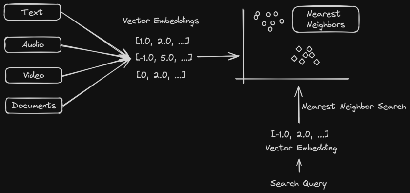
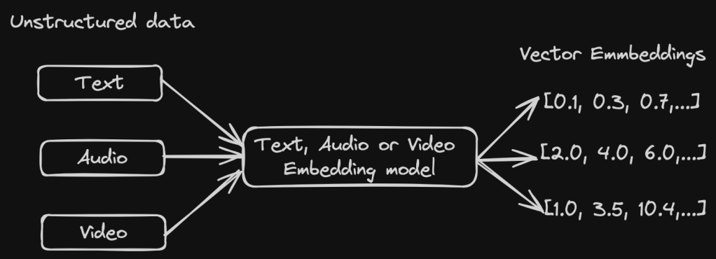
To recap, documents are represented as vector embeddings in a vector space model that captures semantic similarities based on the context. A user query is then converted to a vector embedding and efficient algorithms such as KNN, ANN (Approximate Nearest Neighbor) search are used to find the nearest neighbors to the query. This is where K-Nearest Neighbors algorithm is used where “K” refers to the number of nearest neighbors we want to consider before prediction.

Nearest Neighbor Search

How does KNN work?

KNN works by finding the “K” nearest neighbors in a vector space model. The value of K needs to be chosen carefully to balance between noise and over smoothing. One way is to test for accuracy of the algorithm by evaluating on different values of K using cross-validation where data is divided into training and validation datasets. The validation data set is used to evaluate the performance of the algorithm. A plot with K values and the corresponding error rate can help determine the best K value with the minimum error rate.

KNN finds the nearest neighbors using distance metrics. This can be anything such as Euclidean distance, Manhattan distance etc. We will look at the various distance metrics in detail in the next section.

KNN can be used for both Classification and Regression problems.

  • For Classification problems, the majority class is chosen among the K nearest neighbors.
  • For Regression problems, the average (or the weighted average) of the K nearest neighbors is used.

Distance Metrics

Various distance metrics are used for KNN, Euclidean distance being one of the most common ones.

Euclidean Distance

{\displaystyle d(p,q)={\sqrt {(p_{1}-q_{1})^{2}+(p_{2}-q_{2})^{2}+\cdots +(p_{n}-q_{n})^{2}}}.}
Source: Wikipedia

Euclidean Distance gives the straight line distance between two coordinates in a vector space. This works great for numerical features in the input data.

Manhattan Distance

{\displaystyle \sum _{i=1}^{n}|p_{i}-q_{i}|}
Source: Wikipedia

Manhattan Distance calculates the sum of absolute differences between the vector data points. This is good with categorical features. It is not as sensitive to outliers as Euclidean Distance.

Mikowski Distance

{\displaystyle D\left(X,Y\right)={\biggl (}\sum _{i=1}^{n}|x_{i}-y_{i}|^{p}{\biggr )}^{\frac {1}{p}}.}
Source: Wikipedia

Mikowski Distance is a generalization of the above distances.

  • If p = 1, we get Manhattan Distance
  • If p = 2, we get Euclidean Distance

Hamming Distance

Hamming Distance between two vectors of same length is the number of positions where the corresponding vector values are different. This is suitable for categorical and even binary data.

Cosine Similarity

{\displaystyle {\text{cosine similarity}}=S_{C}(A,B):=\cos(\theta )={\mathbf {A} \cdot \mathbf {B}  \over \|\mathbf {A} \|\|\mathbf {B} \|}={\frac {\sum \limits _{i=1}^{n}{A_{i}B_{i}}}{{\sqrt {\sum \limits _{i=1}^{n}{A_{i}^{2}}}}\cdot {\sqrt {\sum \limits _{i=1}^{n}{B_{i}^{2}}}}}},}
Source: Wikipedia

This is commonly used for high dimensional vector data or text data and it calculates the distance using the cosine of the angle between two vectors.

KNN Algorithm Example for Classification

We have a good understanding of KNN. Now let us look at an actual code example of KNN for a Classification problem.

As a coding exercise, try to implement the averaging functionality for a regression KNN algorithm on your own.

from algorithms.knn import distances

METRICS = {
    "euclidean": distances.EuclideanDistance(),
    "manhattan": distances.ManhattanDistance(),
    "mikowski": distances.MikowskiDistance(),
    "hamming": distances.HammingDistance(),
    "jaccard": distances.JaccardDistance(),
    "cosine": distances.CosineDistance()
}


def get_majority_element(computed_distances):
    """
    Takes an iterable of tuples (distance, class_type)
    and finds the majority class_type
    :param computed_distances: iterable of tuples
    :return: majority element: string
    """
    freq = {}
    for _, class_type in computed_distances:
        if class_type not in freq:
            freq[class_type] = 1
        else:
            freq[class_type] += 1
    return max(freq, key=freq.get)


def knn(training_data, k, distance_metric, test_value):
    """
    Find the k nearest neighbors in training_data for the
    given test value to determine the class type
    :param training_data: Dictionary of class type keys and list of vectors
    as values
    :param k: Integer
    :param distance_metric: string
    :param test_value: query vector
    :return:
    """

    if distance_metric not in METRICS:
        raise ValueError(distance_metric + "is not a valid input")

    distance_calculator = METRICS[distance_metric]
    computed_distances = []

    for class_type, points in training_data.items():
       for point in points:
           distance = distance_calculator.calculate(point, test_value)
           computed_distances.append((distance, class_type))

    # sort the tuples by the computed distance
    computed_distances.sort()
    return get_majority_element(computed_distances[:k])
from abc import abstractmethod, ABC
from math import pow, sqrt

ROUND_TO_DECIMAL_DIGITS = 4

class Distances(ABC):
    @abstractmethod
    def calculate(self, x1, x2):
        pass

class EuclideanDistance(Distances):
    def calculate(self, x1, x2):
        """
        Compute the Euclidean distance between two points.

        Parameters:
        x1 (iterable): First set of coordinates.
        x2 (iterable): Second set of coordinates.

        Returns:
        float: Euclidean Distance
        """
        if len(x1) != len(x2):
            raise TypeError("The dimensions of two iterables x1 and x2 should match")
        return round(sqrt(sum(pow(p1 - p2, 2) for p1, p2 in zip(x1, x2))), ROUND_TO_DECIMAL_DIGITS)

Real World Applications of KNN

KNN is used in a variety of applications such as

  • Recommendation Systems – to recommend the most popular choices among users for collaborative filtering by identifying users with similar behavior.
  • Disease Classification – it can predict the likelihood of certain conditions using majority voting.
  • Semantic Search – to find semantically similar documents or items for a user’s query.
  • Text Classification – spam detection is a good example.
  • Anomaly Detection – It can signify data points that differ from the rest of the data in a system and many many more.

I hope you enjoyed reading about K-Nearest Neighbors algorithm. We will continue to explore various topics related to Semantic Search as well as Search and Ranking in general over the next few weeks.

If you like learning about these types of concepts, don’t forget to subscribe to my blog below to get notified right away when there is a new post 🙂 Have an amazing week ahead!

Posted in Search and Ranking

Introduction to Semantic Search

Semantic search is a type of search that takes into account the meaning and context of a query from a user as opposed to lexical search which only looks for exact keyword match of the query terms.

As an example, when a user searches for the term “football”, we want the search to also consider words such as “soccer”. When “football” is misspelled as “ftball”, we still want to match with “football”.

Semantic search has the ability to dramatically improve the user experience by improving the quality of search results. This is achieved by various Machine Learning models and AI technologies.

Structured Vs Unstructured Data

Structured data is well-defined and is easily searchable whereas unstructured data can be anything such as photos, audio, videos, paragraphs of texts, emails etc and is harder to search through.

Structured data fits well into a storage solution such as a relational database and is searchable using SQL queries but unstructured data does not and needs to be processed using machine learning algorithms to get relevant search results.

As much as 80% of data out there is unstructured. This is important for semantic search because it works on unstructured data which needs to be indexed in a way that it is searchable as efficiently as possible.

Transforming Unstructured Data Using Vector Embeddings

In order for Machine Learning algorithms to process unstructured data to get the most relevant results, this data needs to be represented in a way that the ML models can understand.

This is where Vector Embeddings become useful. Vector Embeddings represent data in numerical form. This opens up a world of computational possibilities on this data. Vector Embeddings transform unstructured data into points in the vector space where similar points get clustered together. This means words, sentences, audio data etc can be represented as vectors which get clustered together in an n-dimension vector space according to their similarity. This is then used by machine learning algorithms to find patterns using which we can do queries that find the most relevant search results.

Vector Embeddings

Here is an example of a 5 dimensional vector embedding. Each point in the vector refers to a feature representing the data.

[1.0, 3.0, 5.0, 7.0, 9.0]

There are various types of embeddings such as word embeddings, graph embeddings, image embeddings etc. The most common type of embeddings used are word embeddings which is used to represent textual data and is used in Semantic Search.

Indexing Vector Data

When data is represented as vector embeddings, it can have high dimensionality based on the number of features used to represent the data. We therefore need a way to efficiently search through large sets of vector embeddings.

Indexing the vector data in the right way helps in efficiently retrieving the most relevant results during search. There are various indexing algorithms proposed for this but a couple of them are highly popular.

Locality Sensitive Hashing (LSH)

This technique is used to do an approximate nearest neighbor search in high dimension vector space. LSH is a hashing based algorithm that will hash similar points to the same or nearby buckets with a high probability so that the search space reduces. Collisions are maximized for similar inputs unlike traditional hashing where we minimize them. This makes it faster to find the approximate nearest neighbors.

Some parameters that need tuning to achieve a good trade off between accuracy and efficiency are hash size, number of hashing functions, number of hash tables etc.

Hierarchical Navigable Small Worlds (HNSW)

HNSW is a graph based data structure that can be used for approximate nearest neighbor search. This works great for high dimensionality vector data since it navigates the graph efficiently for similarity search.

The graph data structure is organized into levels with the bottom layer containing the most data points and each layer above it being a subset of the previous one. The vertices are created such that the likelihood of a graph node appearing in top layers decreases exponentially, which helps keep the graph sparse at higher levels enabling efficient search.

During a search operation, we start at the top most layer and navigate towards the bottom of the graph to find the nearest neighbors that decrease the distance to the input data points. This means we are searching more coarsely at the top instead of having to search the entire graph and keep refining the search as we get to the bottom layer.

HNSW graph

In the example above, we want to find the nearest neighbor of the red dot. So we start at the top most layer at an entry point node and traverse to the neighbor, we then go to the next levels to try and find the nearest neighbor. This is an oversimplification of HNSW works but we will look at this topic in detail on another post.

HNSW are efficient and have good accuracy, thereby being the most popular algorithm for vector similarity search at the moment. HNSW may not suit data that gets frequent updates since reconstructing the graph often is an expensive process.

Searching on Vector Data

Vector Search

Vector search also known as nearest neighbor search is what powers several semantic search use cases. This works efficiently on vector embeddings that we learnt about in the previous section. Since the search query is also represented as a vector, finding the most relevant results would mean searching for the nearest neighbors for the given query data.

The most popular algorithm for doing a nearest neighbor search in kNN – k nearest neighbor search. This provides highly accurate results but it is also computationally intensive. For large language model datasets, this does not scale well. So in these cases, the ANN – Approximate Nearest Neighbor search works much better at the cost of slightly reduced accuracy. We will learn about KNNs and ANNs in future posts on this topic.

Hope you enjoyed learning about semantic search. Let’s continue to explore this topic in more detail.