Posted in Java Programming, Search and Ranking

Build a Simple Apache Lucene Search Application using Java Spring Boot

In this tutorial, we are going to build a bare bones Search Application using Apache Lucene and Java Spring Boot. You will learn the basics of a Lucene Search Application by the time you finish this tutorial.

I have also attached the link to the full GitHub code in case you want to dive deeper into the code right away.

What is Apache Lucene?

Apache Lucene is a powerful Open Source Java library with Indexing and Search capabilities. There is also PyLucene with Python bindings for Lucene Core. Our tutorial will be in Java. Several Search Applications that are widely used in the industry today use Apache Lucene behind the scenes. This includes Elasticsearch, Nrtsearch, Cloudera, Github, Solr etc.

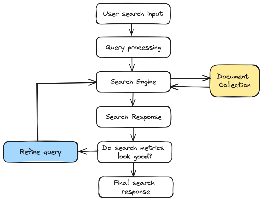
In this tutorial, you will learn to set up a simple Search Application using Apache Lucene in Java Spring Boot which is also an open source tool that makes setting up RESTful applications simple and easy.

Components of a Simple Search Application

Components of a Search Application

Indexer

Inverted Index

Apache Lucene can perform fast full-text searches because of indexes that are built as Inverted Indexes. This is different from a regular index and for each term that appears in a pool of documents, the document ID and the position of that term in the document is stored. This list of doc IDs and positions is called a Postings List. The diagram below shows an example with only the doc IDs for each term. This allows fast look up during query time.

Postings List

Lucene Indexer

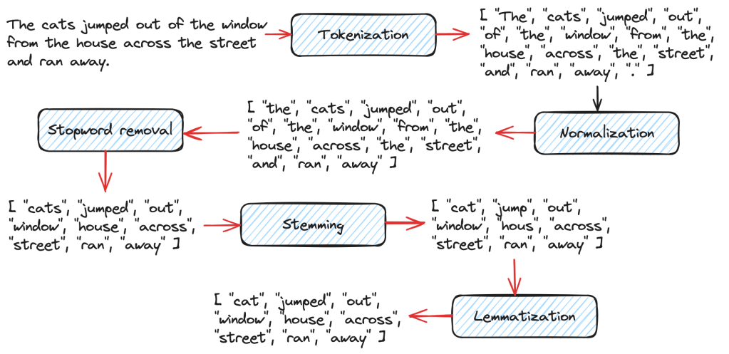
The Lucene Indexer does a list of steps to convert raw text documents into Inverted Indexes. These include text analysis, splitting the text into smaller tokens and other processing such as stop words removal, lemmatization etc. There are several Analyzers available in Lucene based on user and language needs. In this tutorial, we will be using the Lucene StandardAnalyzer.

We will create a Lucene Document object which gets stored in Lucene Indexes from the raw text files. A Search Query in Lucene returns a set of Documents as the result. A Document contains a collection of Fields where each Field is a combination of Field name and a value that can be retrieved at search time using a Query.

In the code example below, we declare the path to the Index Directory. This is where the index files get stored. The Index Directory is a normal file system location on the local device and you will see it being created at the mentioned path once you run the indexing method. We initialize an IndexWriterConfig instance with a Lucene StandardAnalyzer and create an IndexWriter to index all the documents.

Directory indexDirectory = FSDirectory.open(Paths.get(INDEX_DIR));
IndexWriterConfig indexWriterConfig = new IndexWriterConfig(analyzer);
IndexWriter indexWriter = new IndexWriter(indexDirectory, indexWriterConfig);

// The file can be indexed using the IndexWriter as follows.
indexDocument(indexWriter, file);

// Method where the file contents get converted to a Lucene Document object before being indexed.
private void indexDocument(IndexWriter indexWriter, File file) throws IOException {
    Document doc = new Document();
    doc.add(new StoredField("fileName", file.getName()));
    doc.add(new TextField("fileContent", new FileReader(file)));
    indexWriter.addDocument(doc);
}

We map the indexing method to the path /index in our Spring Boot Application running on localhost:8080 which will produce the following output when indexing is done. Only 5 static files are used as Documents to keep things simpler. So this is a GET method in the code example.

Lucene Indexing

Query

Query is the user-facing component of Lucene. A user can send any type of Lucene Query such as a BooleanQuery, TermQuery, PhraseQuery, PrefixQuery, PhraseQuery, FuzzyQuery etc. For our example, we are using a simple Lucene TermQuery.

A TermQuery consists of a field name and a value. Lucene will return the Documents that contain the specific term. The example below from the GET request that is sent to the search application contains the following components.

  • TermQuery – type of Query to map the Search Request to.
  • maxHits – the maximum number of documents to return for the result.
  • fieldName – the name of the Document Field
  • fieldValue – the specific Term to search for in the Lucene Documents.
body: JSON.stringify({
    "type": "TermQuery",
    "maxHits": 4,
    "fieldName": "fileContent",
    "fieldValue": "lucene"
})

We will convert the above Json Query into a Lucene TermQuery using a simple method as shown below.

public Query parseJsonToQuery() {
    return new org.apache.lucene.search.TermQuery(new Term(fieldName, fieldValue));

In this example, we want Lucene to return all Documents (maximum of 4) that contains the term “lucene” in the “fileContent” Field.

Searcher

Searching in Lucene is the process where a user Query is sent as a search request using the Lucene IndexSearcher. See below for the example.

  • IndexSearcher – used to search the single index that we created in the above step.
  • Query – the JSON request is parsed into a TermQuery in this case based on the specified type.
  • maxHits – the maximum number of Documents to return in the search response.
  • ScoreDoc[] – The indexSearcher.search() method returns a list of hits called TopDocs which are the Documents that satisfy the given Query. ScoreDoc contains the doc ID of the hit and the Relevance Score that was assigned by Lucene based on the match criteria of the Documents to the given Query.
@RequestMapping(
    value = "/search",
    method = RequestMethod.POST,
    produces = "application/json; charset=utf-8",
    consumes = MediaType.APPLICATION_JSON_VALUE)
public List<String> search(@RequestBody SearchRequest searchRequest) throws IOException {
    List<String> results = new ArrayList<>();

    Directory indexDirectory = FSDirectory.open(Paths.get(INDEX_DIR));
    IndexReader indexReader = DirectoryReader.open(indexDirectory);
    IndexSearcher indexSearcher = new IndexSearcher(indexReader);

    Query query = searchRequest.parseJsonToQuery();
    int maxHits = searchRequest.getMaxHits();

    ScoreDoc[] hits = indexSearcher.search(query, maxHits).scoreDocs;
    for (ScoreDoc hit : hits) {
      Document doc = indexSearcher.doc(hit.doc);
      results.add(doc.get("fileName"));
    }
    return results;
}

The /search POST request looks something like this.

fetch('http://localhost:8080/search', {
    method: 'POST',
    headers: {
        'Content-Type': 'application/json'
    },
    body: JSON.stringify({
        "type": "TermQuery",
        "maxHits": 4,
        "fieldName": "fileContent",
        "fieldValue": "lucene"
    })
})
.then(response => response.json())
.then(data => console.log(data))
.catch(error => console.error('Error:', error));

To send requests like this to our Spring Boot Application,

  • Go to localhost:8080 on the browser
  • Right click and choose Inspect
  • Go to Console, paste the above code and click Enter.

Alternatively, you can also send CURL requests from your terminal. Examples are linked in the readme document of the Github Repo.

You should see some results as shown below in the Console. Document 2, 5, 4 and 1 were the top ranked results by Lucene.

Searcher Response

The full code can be found on my Github. I highly recommend that you take a look to understand this tutorial well. Feel free to download the project and add more capabilities to your Search Application. One idea is to add support for more types of Lucene Queries.

Hope you enjoyed reading this tutorial on setting up a Simple Lucene Search Application using Java Spring Boot. See you in the next blog post!

Posted in Search and Ranking

Introduction to Information Retrieval

Information Retrieval is the process of finding the most relevant information from a large collection of data (set of documents) for a given user query. Information Retrieval is the back bone of several systems such as

  • Web Search
  • Email Search
  • Library catalogs
  • ChatGPT etc

In this post, we will be learning about the following topics.

  • General Search Process
  • Document Indexing – Inverted Index
  • Text Processing
  • Types of Retrieval Models
  • Metrics to Evaluate Search

General Search Process

The following diagram gives an idea of the overall search process. When a user searches for a certain information, that information is transformed into a query that can be understood and processed by the search engine.

The query is then processed by the search engine to retrieve the most relevant documents from the collection. Certain metrics are used to evaluate the search response and if the results are not satisfactory, we refine the query further and reprocess it.

General search flow

Document Indexing – Inverted Index

In order to retrieve information as fast as possible, we need to index the documents efficiently. We build what is called an “Inverted Index” for fast look up of documents that are most relevant to a search input.

An inverted index is a mapping of the different terms in a large collection to a list of documents in which the term occurs. The document is usually referred to by the document ID aka doc ID. The list of doc IDs is called a postings list. A variable length postings list is used to keep it updated as documents get updated.

Terms and Postings Lists

Text Processing

Before building the inverted index, a number of text processing steps are performed on the documents in order to retrieve information effectively and minimize storing unnecessary words.

Tokenization

This step breaks down the given documents or text into individual words called tokens.

Normalization

At this step, extraneous details such as caps lock, punctuation etc are removed.

Remove Stopwords

There are many words such as “the”, “a” etc which don’t have any significance, so these are removed.

Stemming and Lemmatization

Stemming removes unwanted prefixes and suffixes from words. For ex: running -> run, books -> book.

Lemmatizers on the other hand, transform a word to its language-specific dictionary form. This produces more linguistically accurate words.

Different stages of text processing

Types of Retrieval Models

Boolean Retrieval Model

This model can process Boolean queries that involve Boolean operators such as AND, OR, NOT etc. The inverted index is built based on the presence of terms in documents. This is simple and pretty popular but it cannot process queries that require contextual understanding.

Probabilistic Retrieval Model and BM25

This model ranks the documents based on the probability of their relevance to the search query. Okapi BM25 where BM stands for “Best Matching” is one of the most popular algorithms under the Probabilistic Retrieval Model. It calculates the document scores using various parameters such as term frequency, inverse document frequency, document length normalization etc.

Vector Space Model

In this model, data and queries are transformed into vectors in a multi-dimensional space. The number of dimensions will depend on the features used to represent the data. There are various distance metrics that can be used to compute the distance between points that capture semantic similarity but cosine distance is a popular one. This is a great model to capture contextual information.

Latent Semantic Indexing

This model captures latent semantic relationships between documents and terms using Singular Value Decomposition (SVD) to identify underlying concepts within a body of text. SVD is a technique to reduce dimensionality while preserving contextual information at the same time.

Neural Information Retrieval

NIR can capture complex semantics in text data thereby improving the accuracy and relevance of search. This model uses Neural Networks to retrieve highly relevant documents during search.

Metrics to Evaluate Search

There are two popular metrics to evaluate how good search results are. Although there are many others that we will be looking into in the future, these two are important.

  • Precision – This metric refers to the fraction of documents retrieved by search that are relevant to the user query. This points to the accuracy of the search results. Precision values are between 0 and 1 where 1 means a perfect accuracy score where all the documents were relevant to the search query.
  • Recall – This metric refers to the fraction of relevant documents retrieved by search from the total number of relevant documents in the collection. Recall values also range from 0 to 1 with 1 meaning that all the relevant documents in the collection were retrieved by the search operation.

Hope you enjoyed this Introduction to Information Retrieval post. Let us continue exploring various topics related to Information Retrieval and Semantic Search in future posts. Have a wonderful day!

Posted in AI/ Machine Learning, Search and Ranking, Software Engineering

K-Nearest Neighbors (KNN) Algorithm

We learnt about Semantic Search in my previous post. Here is the link if you missed it. K-Nearest Neighbors is one of the most popular Machine Learning algorithms used in semantic search to find documents or data that is semantically similar to a user’s query.

To recap, documents are represented as vector embeddings in a vector space model that captures semantic similarities based on the context. A user query is then converted to a vector embedding and efficient algorithms such as KNN, ANN (Approximate Nearest Neighbor) search are used to find the nearest neighbors to the query. This is where K-Nearest Neighbors algorithm is used where “K” refers to the number of nearest neighbors we want to consider before prediction.

Nearest Neighbor Search

How does KNN work?

KNN works by finding the “K” nearest neighbors in a vector space model. The value of K needs to be chosen carefully to balance between noise and over smoothing. One way is to test for accuracy of the algorithm by evaluating on different values of K using cross-validation where data is divided into training and validation datasets. The validation data set is used to evaluate the performance of the algorithm. A plot with K values and the corresponding error rate can help determine the best K value with the minimum error rate.

KNN finds the nearest neighbors using distance metrics. This can be anything such as Euclidean distance, Manhattan distance etc. We will look at the various distance metrics in detail in the next section.

KNN can be used for both Classification and Regression problems.

  • For Classification problems, the majority class is chosen among the K nearest neighbors.
  • For Regression problems, the average (or the weighted average) of the K nearest neighbors is used.

Distance Metrics

Various distance metrics are used for KNN, Euclidean distance being one of the most common ones.

Euclidean Distance

{\displaystyle d(p,q)={\sqrt {(p_{1}-q_{1})^{2}+(p_{2}-q_{2})^{2}+\cdots +(p_{n}-q_{n})^{2}}}.}
Source: Wikipedia

Euclidean Distance gives the straight line distance between two coordinates in a vector space. This works great for numerical features in the input data.

Manhattan Distance

{\displaystyle \sum _{i=1}^{n}|p_{i}-q_{i}|}
Source: Wikipedia

Manhattan Distance calculates the sum of absolute differences between the vector data points. This is good with categorical features. It is not as sensitive to outliers as Euclidean Distance.

Mikowski Distance

{\displaystyle D\left(X,Y\right)={\biggl (}\sum _{i=1}^{n}|x_{i}-y_{i}|^{p}{\biggr )}^{\frac {1}{p}}.}
Source: Wikipedia

Mikowski Distance is a generalization of the above distances.

  • If p = 1, we get Manhattan Distance
  • If p = 2, we get Euclidean Distance

Hamming Distance

Hamming Distance between two vectors of same length is the number of positions where the corresponding vector values are different. This is suitable for categorical and even binary data.

Cosine Similarity

{\displaystyle {\text{cosine similarity}}=S_{C}(A,B):=\cos(\theta )={\mathbf {A} \cdot \mathbf {B}  \over \|\mathbf {A} \|\|\mathbf {B} \|}={\frac {\sum \limits _{i=1}^{n}{A_{i}B_{i}}}{{\sqrt {\sum \limits _{i=1}^{n}{A_{i}^{2}}}}\cdot {\sqrt {\sum \limits _{i=1}^{n}{B_{i}^{2}}}}}},}
Source: Wikipedia

This is commonly used for high dimensional vector data or text data and it calculates the distance using the cosine of the angle between two vectors.

KNN Algorithm Example for Classification

We have a good understanding of KNN. Now let us look at an actual code example of KNN for a Classification problem.

As a coding exercise, try to implement the averaging functionality for a regression KNN algorithm on your own.

from algorithms.knn import distances

METRICS = {
    "euclidean": distances.EuclideanDistance(),
    "manhattan": distances.ManhattanDistance(),
    "mikowski": distances.MikowskiDistance(),
    "hamming": distances.HammingDistance(),
    "jaccard": distances.JaccardDistance(),
    "cosine": distances.CosineDistance()
}


def get_majority_element(computed_distances):
    """
    Takes an iterable of tuples (distance, class_type)
    and finds the majority class_type
    :param computed_distances: iterable of tuples
    :return: majority element: string
    """
    freq = {}
    for _, class_type in computed_distances:
        if class_type not in freq:
            freq[class_type] = 1
        else:
            freq[class_type] += 1
    return max(freq, key=freq.get)


def knn(training_data, k, distance_metric, test_value):
    """
    Find the k nearest neighbors in training_data for the
    given test value to determine the class type
    :param training_data: Dictionary of class type keys and list of vectors
    as values
    :param k: Integer
    :param distance_metric: string
    :param test_value: query vector
    :return:
    """

    if distance_metric not in METRICS:
        raise ValueError(distance_metric + "is not a valid input")

    distance_calculator = METRICS[distance_metric]
    computed_distances = []

    for class_type, points in training_data.items():
       for point in points:
           distance = distance_calculator.calculate(point, test_value)
           computed_distances.append((distance, class_type))

    # sort the tuples by the computed distance
    computed_distances.sort()
    return get_majority_element(computed_distances[:k])
from abc import abstractmethod, ABC
from math import pow, sqrt

ROUND_TO_DECIMAL_DIGITS = 4

class Distances(ABC):
    @abstractmethod
    def calculate(self, x1, x2):
        pass

class EuclideanDistance(Distances):
    def calculate(self, x1, x2):
        """
        Compute the Euclidean distance between two points.

        Parameters:
        x1 (iterable): First set of coordinates.
        x2 (iterable): Second set of coordinates.

        Returns:
        float: Euclidean Distance
        """
        if len(x1) != len(x2):
            raise TypeError("The dimensions of two iterables x1 and x2 should match")
        return round(sqrt(sum(pow(p1 - p2, 2) for p1, p2 in zip(x1, x2))), ROUND_TO_DECIMAL_DIGITS)

Real World Applications of KNN

KNN is used in a variety of applications such as

  • Recommendation Systems – to recommend the most popular choices among users for collaborative filtering by identifying users with similar behavior.
  • Disease Classification – it can predict the likelihood of certain conditions using majority voting.
  • Semantic Search – to find semantically similar documents or items for a user’s query.
  • Text Classification – spam detection is a good example.
  • Anomaly Detection – It can signify data points that differ from the rest of the data in a system and many many more.

I hope you enjoyed reading about K-Nearest Neighbors algorithm. We will continue to explore various topics related to Semantic Search as well as Search and Ranking in general over the next few weeks.

If you like learning about these types of concepts, don’t forget to subscribe to my blog below to get notified right away when there is a new post 🙂 Have an amazing week ahead!