Data Structures/ Leetcode – Page 2

Find cheapest flights within K stops

Posted on July 8, 2020July 9, 2020 by Swetha Kannan

There are n cities connected by m flights. We are also given a list with elements containing three pieces of information [u, v, w] where:

Source city: u
Destination city: v
Price to fly from u to v: w

Our goal is to find the cheapest flight ticket from a given source city src to a destination city dst with up to k stops. If no route exists, return -1.

Example 1:
Input:
n = 3, edges = [[0,1,100],[1,2,100],[0,2,500]]
src = 0, dst = 2, k = 1
Output: 200
Explanation:
The graph looks like this:

The cheapest price from city 0 to city 2 with at most 1 stop costs 200, as marked red in the picture.

Solution:

This problem can be re-phrased as trying to find the shortest path between nodes in a weighted graph. Here the nodes are the cities and the weights refer to the flight prices. The simplest graph algorithm to find the shortest path in a weighted graph is Dijkstra’s Shortest Path First algorithm. If this was an unweighted graph, Breadth First Search would have been our ideal choice. This is a good difference to remember. In interviews, the first right move is to model the problem correctly. The next move is to narrow down to the right choice of algorithms.

To solve a graph problem, we have to first construct the graph from the edges. In this problem, for every source city, we store information about the destination cities that we can get to, as well as the corresponding prices. Our constructed graph will look like this.

edges = [[0, 1, 100], [1, 2, 100], [0, 2, 500]]

0: [(1, 100), (2, 500)]
1: [(2, 100)]

How can we make sure to always pick the path with the lowest weight? What kind of data structure always yields the lowest value? If you haven’t guessed it yet, the answer is a min-heap/ priority queue.

The only catch in this problem is the added restriction of having to reach our destination in at most K stops. Therefore, our priority queue contains elements that hold three key pieces of information.

The current node src
The lowest cost to current node
Minimum number of stops to get to the current node

Note that the priority queue will always give us the element with the lowest cost. We will process the queue as long as there are elements left in it or until we reach the destination dst node. This will be our algorithm at each iteration.

Pop the lowest cost element from priority queue. This gives us three values curr_node, curr_cost, curr_stops.
If the curr_node is the same as the destination dst node, return the curr_cost where curr_cost gives the lowest cost with at most K stops to get to the destination.
If the curr_node is not the destination and curr_stops <= K, then we iterate through the edges of this node stored in our graph. Note that each graph vertex may have multiple routes/ edges to different cities.
A neighboring edge contains a vertex v and cost c to get there. We will push (v, cost, K) to the priority queue where cost and K are obtained as follows.
- cost = curr_cost + c
- K = curr_stops + 1

Look at the picture below that walks you through the given example step by step.

Time Complexity: The complexity is defined by the number of pop operations we have to do with the min-heap and the number of edges we process for each graph node. Popping from heap takes logarithmic time, so ignoring duplications in the heap, time complexity will be log V. The graph we constructed is an adjacency matrix representation, so the worst case complexity will be V². The overall complexity is O(V² log V). Note that the heap complexity will be more than log V since we add the same node to the heap more than once to find the shortest path with K stops.

Space Complexity: O(V²) referring to the maximum space taken up by the adjacency matrix. Conservatively, the heap takes O(V) space.

Code:

def findCheapestPrice(self, n: int, flights: List[List[int]], src: int, dst: int, K: int) -> int:

        graph = collections.defaultdict(list)

        for s, d, c in flights:
            graph[s].append((d, c))

        pq = [(0, src, 0)] 

        while pq:
            curr_cost, curr_node, curr_stops = heapq.heappop(pq)

            if curr_node == dst:
                return curr_cost

            if curr_stops <= K:
                for dest, cost in graph[curr_node]:
                    heapq.heappush(pq, (curr_cost + cost, dest, curr_stops+1))

        return -1

Hope you enjoyed reading the solution to this problem 🙂 Have a great day!

Data Structures/ Leetcode, Dynamic Programming, June Leetcoding Challenge

Coin Change – Dynamic Programming

Posted on June 8, 2020June 8, 2020 by Swetha Kannan

We are given an infinite supply of coins of ‘n’ different denominations and a total amount T. We have to find the total number of distinct ways in which we can make up this amount.

Input: amount = 5, coins = [1, 2, 5]
Output: 4
Explanation: There are four ways to make up the amount 5.
5=5
5=2+2+1
5=2+1+1+1
5=1+1+1+1+1

Infinite supply of coins means that we can choose the same coin multiple times in order to make up the total amount 5.

Solution #1: Let’s start with a brute force approach which is to try all the possible combinations from the given coins. Each combination is a subset of coins. For each coin, we can make two different decisions.

If the coin amount does not exceed the total give amount, we can INCLUDE THE COIN in our subset combination and then recursively make a decision on the remaining coins including the current coin, since we can repeatedly choose the same coin to get T.
Another option is to EXCLUDE THE COIN and create a new subset combination with the remaining coins.

The above points make up the core algorithm of this problem. Let’s say the total amount is T and C is the current denomination of the coin that we are processing. Then,

If we include the first coin C, the sum left to make up to T will be T – C and we process the list coins[0…n-1] since we are allowed to select the same coin again.
If we exclude the first coin, the sum left to make up to T will remain the same and we will process the list coins[1…n-1].

This gives way to a recursion tree as shown below.

Time Complexity: This algorithm has exponential time complexity O(2^C+T) where C is the total coins we are given and T is the total amount. This is because for each coin c and amount t, we have to make two decisions ie., branch into two recursive sub-problems of including and excluding the coin.

Space Complexity: O(2^C+T) since the recursion will use stack space that is as deep as the recursion tree.

Code for solution #1:

def change(self, amount: int, coins: List[int]) -> int:
    
    def countHelper(coins, totalAmount, coinIndex):
        
        # If the amount is 0, there is only one way to make this
        # Just exclude the coin
        if totalAmount == 0:
            return 1
        
        n = len(coins)
        # No coins left or all coins have been processed
        if n == 0 or currentIndex >= n:
            return 0
        
        includeCoinSum = 0
        if coins[coinIndex] <= totalAmount:
            includeSum = countHelper(coins, totalAmount - coins[coinIndex], coinIndex)
            
        excludeCoinSum = countHelper(coins, totalAmount, coinIndex + 1)
        
        return includeCoinSum + excludeCoinSum
    
    return countHelper(coins, amount, 0)

Solution #2: It’s pretty clear that an exponential algorithm is not efficient. This is when dynamic programming comes into action. Why is this problem a good candidate for dynamic programming?

Overlapping sub-problems: As we branch down the tree, we saw in the recursion tree image that we compute the total number of ways for some coin c and amount t repeatedly. If the tree size grows, the repetitions will be even higher. This means we can cache the results of a sub-problem and then re-use it the next time we want to compute the same. This is called memoization technique.

Optimal sub-structure: In any given problem, if we are able to compute the optimal solution for a larger problem by computing the optimal results for its smaller sub-problems, then it follows the optimal sub-structure property.

How can we choose what to memoize? To figure this part out, we look at the two variables that are constantly changing state in solution #1 code. This is the coinIndex and the totalAmount values which keep changing during every recursive call. So we store the count value (number of ways) to make an amount totalAmount with the coin at coinIndex during each recursive call. Our memoization array is a 2D array dp[len(coins)][totalAmount + 1] and the number of sub-problems that we need to solve will be C * T ie., for each grid in the 2D array.

Time Complexity: O(C * T) to compute all the sub-problems.

Space Complexity: O(C * T) for the dp array and the recursion costs another O(C) stack space, which adds up to O(C * T + C). So the overall space complexity will be O(C * T).

Code for solution #2:

def change(self, amount: int, coins: List[int]) -> int:
    
    def countHelper(dp, coins, totalAmount, coinIndex):
        
        # If the amount is 0, there is only one way to make this
        # Just exclude the coin
        if totalAmount == 0:
            return 1
        
        n = len(coins)
        # No coins left or all coins have been processed
        if n == 0 or currentIndex >= n:
            return 0
        
        if dp[coinIndex][totalAmount] != -1:
            return dp[coinIndex][totalAmount]
        
        includeCoinSum = 0
        if coins[coinIndex] <= totalAmount:
            includeSum = countHelper(dp, coins, totalAmount - coins[coinIndex], coinIndex)
            
        excludeCoinSum = countHelper(dp, coins, totalAmount, coinIndex + 1)
        
        dp[coinIndex][totalAmount] = includeCoinSum + excludeCoinSum
        return dp[coinIndex][totalAmount]
    
    dp = [[-1 for _ in range(amount+1)] for _ in range(len(coins))]
    
    return countHelper(dp, coins, amount, 0)

The above approach is called top down dynamic programming. This is because we start with the larger problem and recursively break it down into smaller sub-problems and compute their results. We can avoid recursion by approaching this problem bottom-up. In this case, we compute the results of sub-problems before using them to compute the larger problem. This method is called tabulation.

Solution #3:

We can use the same 2D array dp[len(coins)][totalAmount + 1] to populate the sub-problem results but this time we start from the smallest sub-problem. For this to make sense, we need to understand what a single sub-problem in this array means. dp[c][t] means the total number of ways to make up an amount t by including or excluding the coin at index c.

When we exclude a coin at index c, we can make a total t using dp[c – 1][t] number of ways. We use the coins up until the index c – 1 to make the amount t but we skip the coin at c.
When we include the coin at index c, we have to subtract its value from the total amount t ie., dp[c][t – coins[c]]

Adding the above two results gives the result for dp[c][t] ie. the total number of ways to make t using the coins up until index c.

dp[c][t] = dp[c – 1][t] + dp[c][t – coins[c]]

The dp array contains the following values for the given problem. Our answer is in the bottom right grid of the dp array when we compute dp[C][T] using all the sub-problems.

Time Complexity: O(C * T) to populate the dp array.

Space Complexity: O(C * T) for the 2D array.

Code for the above solution:

def change(self, amount: int, coins: List[int]) -> int:

    if not amount:
        return 1

    if not coins:
        return 0

    n = len(coins)
    dp = [[0 for i in range(amount+1)] for _ in range(n)]

    for i in range(n):
        dp[i][0] = 1

    for c in range(n):
        for t in range(1, amount+1):
            dp[c][t] = dp[c-1][t]

            if coins[c] <= t:
                dp[c][t] += dp[c][t - coins[c]]

    return dp[n-1][amount]

Hope you enjoyed learning how to solve the coin change problem using dynamic programming. Have a great day!

Arrays and Strings, Data Structures/ Leetcode, June Leetcoding Challenge

Queue Reconstruction by Height

Posted on June 6, 2020June 7, 2020 by Swetha Kannan

We are given a list of people described by height h and a number k. k refers to the number of people in front of this person who are of height greater than or equal to their height. We have to write an algorithm to reconstruct the queue.

The number of people will be less than 100.

Input:
[[7,0], [4,4], [7,1], [5,0], [6,1], [5,2]]

Output:
[[5,0], [7,0], [5,2], [6,1], [4,4], [7,1]]

Explanation:

[7, 0] – Height = 7 and there should be 0 people equal in height or taller in front of this person

[4, 4] – Height = 4 and there should be 4 people equal in height or taller in front of this person

[7, 1] – Height = 7 and there should be 1 people equal in height or taller in front of this person

[5, 0] – Height = 5 and there should be 0 people equal in height or taller in front of this person

[6, 1] – Height = 6 and there should be 1 people equal in height or taller in front of this person

[5, 2] – Height = 5 and there should be 2 people equal in height or taller in front of this person

Solution:

There are two elements in each list item which is the height and k.

Input = [[7,0], [4,4], [7,1], [5,0], [6,1], [5,2]]

Output = [[5,0], [7,0], [5,2], [6,1], [4,4], [7,1]]

Let’s manually try to place the people in a queue. The given list looks like this.

We first take the tallest person and place them in the queue according to their index value. If two people have the same index value, then we give priority to the person who is shorter. We will see why in a bit. So the queue will look like this after placing [7, 0] and [7, 1].

Next, we pick the next tallest person in queue [6, 1]. When we try to place them in the index 1, there is already a person of height 7 there. In this case, we need to place the person with the shorter height in front because they should have only 1 more person who is of equal height or is taller than them. We insert this person in the queue before [7, 1]. The queue will now look like this.

We can pick the next tallest person with height 5. We can place [5, 0] before placing [5, 2] since the lower index person gets priority. 0th index already has a person of height 7, but we will push them back and insert [5, 0] to let the shorter person be in the front. The queue will now look like this.

Let’s continue doing this for the left out elements and we will get the following.

The code for this algorithm involves two steps:

Arrange people in descending height. When there is a tie in height, give priority to the one with the lower index.
Insert people according to their indexes into a new queue. When there is a tie in index, give priority to the one with the lower height.

Time Complexity: O(NlogN) for sorting and O(N) to insert an element into a list, so the overall complexity to insert N elements will be O(N²).

Space Complexity: We will do the sorting in place and the result queue need not be considered as extra space, so space complexity is O(1).

Code for the above solution:

def reconstructQueue(self, people: List[List[int]]) -> List[List[int]]:

    # sort people by descending height and ascending index k
    people.sort(key = lambda x: (-x[0], x[1]))

    results = [] * len(people)

    for p in people:
        results.insert(p[1], p)

    return results

Hope you enjoyed reading this post. Have a great day!

Arrays and Strings, Data Structures/ Leetcode, June Leetcoding Challenge

Random pick with weight – a probability problem

Posted on June 5, 2020June 7, 2020 by Swetha Kannan

Today’s problem is a very interesting one but is usually worded poorly in most places.

We are given an array W of positive integers where W[i] refers to the weight of index i. We have to write a function called pickIndex which will randomly pick an index proportional to its weight. Let’s look at an example to understand this better.

W = [1, 2, 3, 4, 5]

In the above case the weights are as follows.

W[0] = 1

W[1] = 2

W[2] = 3

W[3] = 4

W[4] = 5

How do we randomly pick an index proportional to its weight?

The weights of all the indexes in the array sum to 15 (1 + 2 + 3 + 4 + 5).

For index i = 0 with weight = 1, we have to pick this index once out of 15 times

For index i = 4 with weight = 5, we have to pick this index five out of 15 times

The bottomline line is that the indexes with the higher weights should have high probability of being picked, in this case that probability is:

P(i) = W[i] / sum(W)

ie., for index = 4 P(4) = 5/ 15 = 1/ 3.

Solution #1:

For probability problems, one of the foremost things we need is a sample space. Let’s simulate this using a generated array with 15 entries where each entry corresponds to an index in the array and appears W[i] number of times. For example, the index 4 should appear W[4] = 5 times in the array.

Sample space = [0, 1, 1, 2, 2, 2, 3, 3, 3, 3, 4, 4, 4, 4, 4]

If we are to pick a number randomly from the above list, we have solved the problem of picking a random index proportional to its weight.

Time Complexity: The time complexity will be O(sum(W)) to generate the sample space array.

Space Complexity: The simulated array will cost us O(sum(W)) extra space.

Code for solution #1:

class Solution(object):

    def __init__(self, w: List[int):

        totalSum = sum(w)
        table = [0] * totalSum
        
        i = 0
        for j in range(0, len(w)):
            for k in range(i, i + w[j]):
                table[k] = j
            i = i + w[j]
            
        self.size = len(table)
        self.table = table
        

    def pickIndex(self) -> int:
        randomIdx = random.randint(0, self.size - 1)
        
        return self.table[randomIdx]
        

# Your Solution object will be instantiated and called as such:
obj = Solution(w)
param_1 = obj.pickIndex()

The above solution is extremely memory intensive since we generate an array that’s mostly larger than the input array itself to simulate the sample space.

Solution #2:

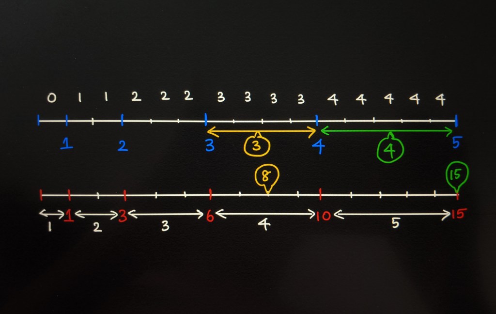
The total sum of our weights sum(W) is 15. If we had to draw a line and divide it according to the given weights ranging from 1 to 15, how would that look like?

W = [1, 2, 3, 4, 5]

sample_space = [0, 1, 1, 2, 2, 2, 3, 3, 3, 3, 4, 4, 4, 4, 4]

Instead of generating an entirely new array with the repeated indexes, we can calculate the prefix sums for each index. The formula to find the prefix sum of W[i] is shown below.

W[i] = W[i] + W[i-1]

Then our prefix array will look like this.

W = [1, 3, 6, 10, 15]

The total weight 15 is the length of our sample space. We will first generate a random number between 1 and 15.

randIndex = random.randint(1, maxWeight)

Let’s say that the randIndex returns 8. This index falls in the range (6 – 10]. So we return the index filling up this range which is 3.

If the randIndex returns 15, this number falls in the range (10 – 15]. So we return the index filling up this range which is 4.

We find this range using linear search on the prefix sum W array. All we have to find a value such that value <= randIndex which indicates that it has fallen in that particular range. In that case, we return the index of this value.

Time Complexity: O(N) to calculate prefix sum and O(N) to find the randIndex value in the prefix sum array. This means the pickIndex function call runs in O(N) time.

Space Complexity: O(1) since we are not using any extra space.

Code for solution #2:

class Solution:

    def __init__(self, w: List[int]):

        # Calculate the prefix sums
        w = list(itertools.accumulate(w))
        self.w = w

        if self.w:
            self.maxWeight = self.w[-1]
        else:
            self.maxWeight = 0

    def pickIndex(self) -> int:

        randIndex = random.randint(1, self.maxWeight)

        for i, prefixSum in enumerate(self.w):
            if randIndex <= prefixSum:
                return i

        return 0
        
#Your Solution object will be instantiated and called as such:
obj = Solution(w)
param_1 = obj.pickIndex()

Solution #3:

In the above solution pickIndex() runs in O(N) time and it’s basically doing a linear search in the array to find the range of the randIndex. We can improve the time complexity using binary search.

In the binary search algorithm, if our randIndex value matches an entry in the prefix sums array, we return that index. Else we return the index of a value which is <= randIndex. This is basically a binary search to find a number N such that N <= target.

Time Complexity: O(logN) to pick the index.

Space Complexity: O(1)

Code for solution #3:

class Solution(object):

    def __init__(self, w: List[int]):
  
        w = list(itertools.accumulate(w))
        self.w = w

        if self.w:
            self.maxWeight = self.w[-1]
        else:
            self.maxWeight = 0
          
    
    def pickIndex(self) -> int:
  
        randIndex = random.randint(1, self.maxWeight)
        
        # Binary search for randIndex
        left = 0
        right = len(self.w) - 1
        
        while left <= right:
            mid = (left + right) / 2
            
            if self.w[mid] == randIndex:
                return mid
            
            if self.w[mid] < randIndex:
                left = mid + 1
            else:
                right = mid - 1
                
        return left
               
# Your Solution object will be instantiated and called as such:
obj = Solution(w)
param_1 = obj.pickIndex()

Solution #4 (Optional):

The code in solution #3 can be written in a very pythonic way using built-in functions as shown below. The time and space complexity will be the same.

Python’s bisect.bisect_left() returns an insertion point i that partitions the array into two halves such that all(val < randIndex for val in w[left : i]) for the left side and all(val >= randIndex for val in a[i : right]) for the right side. Read more here.

class Solution:
    def __init__(self, w: List[int]):
        self.w = list(itertools.accumulate(w))

    def pickIndex(self) -> int:
        return bisect.bisect_left(self.w, random.randint(1, self.w[-1]))
        
#Your Solution object will be instantiated and called as such:
obj = Solution(w)
param_1 = obj.pickIndex()

Hope you learnt to methodically approach the random pick with weight problem. Have a nice day!

Data Structures/ Leetcode, June Leetcoding Challenge, Trees

[Problem Solving] Invert a Binary Tree

Posted on June 1, 2020June 23, 2024 by Swetha Kannan

We are given a binary tree as shown below.

Let’s observe the given tree and compare it with the output. What do we notice?

The left child of a node becomes the right child and vice versa. So we start at the root node and invert the left and right children.

     1
   /   \
  2     3

becomes

     1
   /   \
  3     2

We then invert the left and right sub-trees starting at each of those children. This leads to a naturally recursive approach.

     1
   /   \
  3     2
 / \   / \
6   7 4   5

becomes

     1
   /   \
  3     2
 / \   / \
7   6 5   4

An intuitive way to solve most tree problems is to use recursion. Now we have to decide a few things before coding.

Base case:

Here, the base case would be a NULL node. We simply return at that point since there are no nodes left to invert.

Recursive strategy:

Our recursive strategy involves the following steps.

Invert the left and right child of current node
Recursive call to invert the left sub-tree starting at the left child
Recursive call to invert the right sub-tree starting at the right child

Time Complexity: We will end up visiting each node in the tree, so the time complexity will be O(N) where N is the number of nodes in the tree.

Space Complexity: In recursion problems, an internal stack is used to temporarily hold elements, so the space complexity will be O(H) where H is the height of the tree. This is because as we recurse over left and right sub-trees, the function calls will go as deep as the tree height. In the worst case, H -> N, so the overall space complexity will be O(N) where N is the number of nodes in the tree.

Code for the above solution:

class TreeNode:
    def __init__(self, val=0, left=None, right=None):
        self.val = val
        self.left = left
        self.right = right

def invertTree(self, root: TreeNode) -> TreeNode:

    def invertTreeHelper(root):

        if not root:
            return

        root.left, root.right = root.right, root.left
        invertTreeHelper(root.left)
        invertTreeHelper(root.right)

    invertTreeHelper(root)
    return root

Testing:

These are some of the cases that are good to test for tree problems.

Given test case: [1,2,3,4,5,6,7]
Empty tree: []
No children: [1]
No right child: [1, 2]
Right skewed tree: [1,null,2,null,3,null,4,null,5,null,6,null,7]
Left skewed tree: [1,2,null,3,null,4,null,5,null,6,null,7]

Want to try to solve this problem? https://leetcode.com/problems/invert-binary-tree/

Hope you learnt how to invert a binary tree. Have a great day!

Arrays and Strings, Data Structures/ Leetcode

[Problem Solving] Spiral Matrix

Posted on May 27, 2020June 23, 2024 by Swetha Kannan

Given a matrix of m x n elements, return the elements in spiral order.

[
 [ 1, 2, 3 ],
 [ 4, 5, 6 ],
 [ 7, 8, 9 ]
]

Output: [1,2,3,6,9,8,7,4,5]

This problem is quite popular and is frequently asked during interviews.

Solution: To traverse the matrix in spiral order, we have to go along the boundaries starting from the top left element at i = 0, j = 0 where i, j represent the row and column indexes respectively. Let’s view the matrix as a collection of layers. Once we complete the outermost layer, we have to keep traversing the inner layers until no element is left to be visited. We can think of this as traversing multiple matrices in spiral order layer by layer.

What are some things to remember while traversing?

We need some indexes to track our traversal. A straightforward approach is to have four indexes to keep track of the four boundaries of the matrix. These will be called left, right, top and bottom.
We will be using a while loop to add elements to a results array as long as left < right and top < bottom. This indicates that there are still elements left to traverse.
Inside the while loop, we will be using four for loops to traverse each boundary.
Avoid adding duplicate elements when changing directions ie., once we finish traversing a row [1, 2, 3, 4, 5], we have to increment the row index to avoid adding 5 again during the right most column traversal. Similarly, right and bottom pointers should be decremented upon completing their respective boundary traversals.
This problem code is nothing fancy but a matter of writing clear code without getting confused with the indices. The best way to get it right is to write the for loops as you traverse an example asymmetric matrix. This is because, a symmetric matrices usually do not help us handle edge cases in matrix problems.
One corner case for this problem is when we are traversing a column matrix as shown below where m = 4, n = 1.

In this case, we first initialize these variables.

top = 0
bottom = m #4
left = 0
right = n #1

Top boundary: row = top = 0, col = left to right [0, 1). Results = [1]. Increment top pointer, top = 1.

Right boundary: row = top to bottom [1, 4), col = right – 1 = 0. Results = [ 1, 2, 3, 4]. Decrement right pointer, right = 0.

Now after the above two for loops, we are done traversing the entire matrix. But the next traversal will add duplicate elements to the results.

Bottom boundary: row = bottom – 1 = 3, col = right – 1 to left – 1 [0, -1). Results = [1, 2, 3, 4, 4]

This will attempt to traverse the bottom element 4 again. So right after traversing top and right boundaries, we have to always check whether left < right and top < bottom condition still holds true. In this case top < bottom since 1 < 4 but left = right since 0 = 0 indicating that we are about to traverse a boundary again.

Time Complexity: We will end up visiting each element of the matrix, so time complexity will be O(M * N).

Space Complexity: Constant variables are used to track boundaries, so no additional space is being used. The space complexity will be O(1).

Code:

def spiralOrder(self, matrix: List[List[int]]) -> List[int]:
        
        if not matrix or not matrix[0]:
            return []
        
        m, n = len(matrix), len(matrix[0])
        top, bottom = 0, m
        left, right = 0, n
        
        results = []
        
        while top < bottom and left < right:
            
            # traverse top boundary
            for i in range(left, right):
                results.append(matrix[top][i])
            top += 1
                
            # traverse right boundary
            for i in range(top, bottom):
                results.append(matrix[i][right-1])
            right -= 1
            
            if top < bottom and left < right:
                # traverse bottom boundary
                for i in range(right - 1, left - 1, -1):
                    results.append(matrix[bottom-1][i])
                bottom -= 1

                # traverse left boundary
                for i in range(bottom - 1, top - 1, -1):
                    results.append(matrix[i][left])
                left += 1
            
        return results

Testing: The following cases are good to test for matrix problems.

Empty matrix: []
Empty rows: [[]]
Single value matrix: [[1]]
Two element matrix: [[1, 2]]
Column matrix: [[1,2,3,4]]
Row matrix: [[1],[2],[3],[4]]
Symmetric matrix: [[1,2,3, 4],[4,5,6, 8], [9,10,11,12],[13,14,15,16]]
Asymmetric matrix: [[1,2,3, 4],[4,5,6, 8]]

Want to try solving this problem? https://leetcode.com/problems/spiral-matrix/

Hope you enjoyed this post on traversing a matrix in spiral order. Have a great day!

Arrays and Strings, Data Structures/ Leetcode, Matrix problems

[Problem Solving] Diagonal Traverse

Posted on May 25, 2020June 23, 2024 by Swetha Kannan

Given a matrix of M x N elements, return the elements in diagonal order as shown below.

[
 [ 1, 2, 3, 4 ],
 [ 5, 6, 7, 8 ],
 [ 9, 10, 11, 12 ],
 [13, 14, 15, 16 ]
]

Output: [1, 2, 5, 9, 6, 3, 4, 7, 10, 13, 14, 11, 8, 12, 15, 16]

Solution #1: To begin with, let’s ignore the part where alternate diagonal elements need to be reversed. Let’s try to traverse the matrix as shown above in image 2.

We see that a diagonal always starts either from the top row or the last column of elements. If we are given the starting point of a diagonal, how can we get to the next diagonal element?

For example, let’s say we are at 4 which is at (r = 0, c = 3) where r and c indicate the row and column indexes respectively. To get to the next element, we have to move one row down and one column to the left, ie., r = 1, c = 2. To generalize:

next_r = r + 1, next_c = c – 1

To match the expected results where alternate diagonal elements are reversed in order, we can collect the diagonal elements and reverse the order of alternate diagonals before adding to the results. The code below is an intuitive way of solving this problem.

def findDiagonalOrder(self, matrix: List[List[int]]) -> List[int]:
        
        if not matrix or not matrix[0]:
            return []
        
        m, n = len(matrix), len(matrix[0])
        results = []
        row, col = 0, 0
        
        while row < m and col < n:
            
            temp = []
            
            # To collect all elements of a diagonal, keep going one row down and column 
            # to the left until we hit matrix boundaries
            i, j = row, col
            while i < m and j >= 0:
                temp.append(matrix[i][j])
                i += 1
                j -= 1
                
            # Reverse the order for alternate diagonals
            if (row + col) % 2 == 0:
                results.extend(temp[::-1])
            else:
                results.extend(temp)
                
            # Set row, col to traverse the next diagonal
            if col < n - 1:
                col += 1
            else:
                row += 1
                
        return results

Time Complexity: O(M*N) where M is the number of rows and N is the number of columns in the matrix

Space Complexity: The additional space used in this solution is the temp array which holds the diagonal elements. The largest diagonal of a matrix has min(M, N) elements, so space complexity is O(min(M, N)).

Testing: When it comes to matrix problems, make sure to test the following cases.

Empty matrix: []
Empty rows: [[]]
Single value matrix: [[1]]
Two element matrix: [[1, 2]]
Column matrix: [[1,2,3,4]]
Row matrix: [[1],[2],[3],[4]]
Symmetric matrix: [[1,2,3, 4],[4,5,6, 8], [9,10,11,12],[13,14,15,16]]
Asymmetric matrix: [[1,2,3, 4],[4,5,6, 8]]

Solution #2: The above solution is perfectly acceptable. If you notice the indices of diagonal elements, they all sum to the same number. Remember this pattern as it might come handy while manipulating diagonal elements of a matrix.

Keeping this in mind, here is an alternate solution to this problem where we use the sum of indices as keys in a dictionary to store values belonging to a particular diagonal.

import collections

def findDiagonalOrder(self, matrix: List[List[int]]) -> List[int]:
        
        if not matrix or not matrix[0]:
            return []
        
        m, n = len(matrix), len(matrix[0])
        elements = collections.defaultdict(list)
        results = []
    
        for i in range(m):
            for j in range(n):
                elements[i+j].append(matrix[i][j])
                
        for k, v in elements.items():
            if k % 2 == 0:
                results.extend(v[::-1])
            else:
                results.extend(v)

        return results

Time Complexity: O(M*N)

Space Complexity: O(M*N)

Want to try solving this problem? https://leetcode.com/problems/diagonal-traverse/

Hope you enjoyed solving the diagonal traverse problem. Have a great day!

Arrays and Strings, Data Structures/ Leetcode

[Problem Solving] Plus one to array

Posted on May 23, 2020June 23, 2024 by Swetha Kannan

Given a non-empty array of digits representing a non-negative integer, plus one to the integer. The digits are stored such that the most significant digit is at the head of the list, and each element in the array contain a single digit. You may assume the integer does not contain any leading zero, except the number 0 itself.

Examples:

[1, 2, 3] should return [1, 2, 4]
[9, 9] should return [1, 0, 0]

Solution: When we add 1 to a single digit number, there are two outcomes. It can either remain a single digit number or results in 10. If the result is 10, we have to store 0 in the index i and propagate the carry 1 to the previous index i-1.

Let’s traverse the array from the end and add one to the value at index i.

If the value becomes 10, store 0 in nums[i] and continue traversing the array
Otherwise, add one to the value at nums[i] and return the array

Time Complexity: Since we traverse the array once, O(N)

Space Complexity: No additional space is used, so O(1)

def plusOne(self, digits: List[int]) -> List[int]:
        
        for i in range(len(digits)-1, -1, -1):
            
            if digits[i] + 1 == 10:
                digits[i] = 0
            else:
                digits[i] += 1
                return digits
            
        return [1] + digits #handle the case where all digits become 9

Testing: For most problems it’s good to test the following cases.

Empty array: []
Single value array: [1]
Array with two values: [1, 8]
A random array: [1, 2, 3, 4]

In this problem, there are two important cases to test. When the last digit is 9 and when all the digits are 9.

[1, 9]
[9] or [9, 9] or [9, 9, 9]

Want to try solving this problem? https://leetcode.com/problems/plus-one/

Hope you enjoyed this simple approach to the plus one problem. Have a great day!

Arrays and Strings, Data Structures/ Leetcode

[Problem Solving] Find Pivot Index

Posted on May 23, 2020June 23, 2024 by Swetha Kannan

Let’s say we are given an array of integers and we want to find a pivot index such that the sum of numbers to the left of this index equals the sum of numbers to the right.

Example: [1, 7, 3, 6, 5, 6]

1 + 7 + 3 = 5 + 6 = 11. In this example, the pivot value is 6, whose array index is 3. If no such index exists, return -1.

Solution #1: To get started with a brute force approach, let’s consider each number as a pivot and calculate the left and right side sums until they equal each other.

Pivot = 1, pivotIndex = 0, leftSum = 0, rightSum = 27

Pivot = 7, pivotIndex = 1, leftSum = 1, rightSum = 20

Pivot = 3, pivotIndex = 2, leftSum = 8, rightSum = 17

Pivot = 6, pivotIndex = 3, leftSum = 11, rightSum = 11. Voila!! Here leftSum = rightSum, so return 3 as the answer.

Time Complexity: A worst case scenario is when we have to traverse the entire array and the pivot index is the last index (n-1) of the array which will be O(N). Calculating left and right side sums adds another O(N) and so it will be an O(N²) algorithm. To improve our algorithm efficiency, we have to try to do this in linear time. In the previous approach, calculation of leftSum added to increased complexity, how can we optimize this part? What if we had access to the leftSum and rightSum values in advance?

Solution #2: Let’s pre-calculate the leftSum and rightSum values for each pivot and store these values in two arrays.

[1, 7, 3, 6, 5, 6]

leftSums = [0, 1, 8, 11, 17, 22, 28]

rightSums = [27, 20, 17, 11, 6, 0]

In leftSums and rightSums, we need to find the index whose values are equal, in this case it’s 11 ie., leftSums[3] = rightSums[3].

Time Complexity: In Solution #2, our time complexity will go down from O(N²) to O(N) since we use pre-calculated sum values to find the pivot index ie., O(N) for pre-calculation plus another O(N) while traversing to find pivot index .

Space Complexity: Using two extra arrays to pre-compute values adds additional 2N space. So the overall space complexity will be O(N).

Code for Solution #2:

def pivotIndex(self, nums: List[int]) -> int:
        
        if not nums:
            return -1
        
        n = len(nums)
        leftSums, rightSums = [0] * n, [0] * n
       
        for i in range(1, n):
            leftSums[i] = leftSums[i-1] + nums[i-1]
            
        for i in range(n-2, -1, -1):
            rightSums[i] = rightSums[i+1] + nums[i+1]
            
        for i in range(n):
            if leftSums[i] == rightSums[i]:
                return i
            
        return -1

Slight improvement on space complexity:

Anytime we are traversing an array both ways and then iterating it all over again, it’s possible to eliminate one of the traversals and calculate values on the fly. In the above code snippet, the following chunks of code are kind of doing the same thing, let’s try to avoid code duplication.

for i in range(1, n):
    leftSums[i] = leftSums[i-1] + nums[i-1]

for i in range(n):
    if leftSums[i] == rightSums[i]:
        return i

We can replace the above two blocks by calculating leftSum on the fly as shown below.

for i in range(0, n):

    if i > 0:
        leftSum += nums[i-1]
    if leftSum == rightSums[i]:
        return i

Time Complexity: O(N)

Space Complexity: O(N)

Testing: For array problems like these, it’s important to test the following cases.

Empty array: [] => returns -1
Single value array: [1] => returns 0
Double value array: [1, 2] => returns -1
A random array: [2, 3, 4, 5] => returns 2
All given test cases in the problem statement
Arrays that have one pivot index: [1, 7, 3, 6, 5, 6] => returns 3
Arrays that have more than one pivot index: [1, 0, 1, 0] => returns 0
Arrays with no pivot index: [1, 2, 3, 4] => returns -1

Can we do better? Yes!

Solution #3: Introducing prefix sum

If we are given the leftSum of a pivot, what else do I need to get the rightSum? The total sum of the array.

Example: [1, 7, 3, 6, 5, 6]

totalSum = 1 + 7 + 3 + 6 + 5 + 6 = 28

pivot = 7, pivotIndex = 1, leftSum = 1, rightSum = 28 – 1 – 7 = 20

pivot = 6, pivotIndex = 3, leftSum = 11, rightSum = 28 – 11 – 6 = 11

To generalize, rightSum(i) = totalSum – leftSum – nums[i]. Now let’s alter the code accordingly.

def pivotIndex(self, nums: List[int]) -> int:
        
        if not nums:
            return -1
        
        n = len(nums)
        leftSum = 0
        totalSum = sum(nums)
        
        for i in range(n):
            if leftSum == totalSum - leftSum - nums[i]:
                return i
            
            leftSum += nums[i]
            
        return -1

Time Complexity: O(N) for calculation sum of nums, O(N) for finding pivot index, so the overall time complexity will be O(N).

Space Complexity: O(1) since we use constant space to store totalSum and leftSum values.

Want to solve this problem? https://leetcode.com/problems/find-pivot-index/

Hope you enjoyed this step by step approach to iteratively improve upon a solution for a problem. Have a great day!