Search and Ranking

Fundamentals of a Distributed Search Infrastructure

Posted on June 20, 2024 by Swetha Kannan

Almost all of the apps that we use regularly have a search bar to retrieve results relevant to our search terms – Google, Yelp, Amazon, YouTube etc. As the traffic to these websites scale up, the corresponding Search Backend Infrastructure needs to be able to handle that volume of incoming traffic successfully while ensuring fast and efficient user experience.

We need a Distributed Search Infrastructure to handle these large-scale operations where the Indexing and Search workload is distributed across multiple servers or nodes. This ensures high Availability, Scalability and Low Latencies compared to a system with only server.

Popular Distributed Search Infrastructures

E-Commerce Platforms – Amazon, Etsy etc
Social Media – Instagram, YouTube, TikTok etc
Web Search – Google, Bing etc
Enterprise Search – Document search etc

Distributed Cluster Architecture

A distributed search cluster contains a group of nodes. Different nodes perform different functions. For example, in Elasticsearch

Master Node – this controls an Elasticsearch cluster responsible for many cluster level operations such as creation, deletion of indexes etc.
Data Node – this is where the inverted index containing the search data lives.
Client Node – this is used for routing the incoming search requests to other clusters.

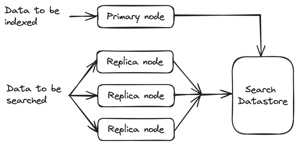
There are other search infrastructures such as Nrtsearch where Indexing and Search is split across different sets of nodes.

Primary – single node that does all the indexing.
Replica – one to several nodes that serve all the search traffic. The number of replicas can be scaled horizontally based on the traffic.

Distributed Search Infrastructure – Design Considerations

Scalability, Reliability, Availability and Performance are some of the crucial aspects to design a Distributed Search Infra.

Scalability

Horizontal Vs Vertical Scaling

In Horizontal Scaling, more servers are added to an existing distributed search infra to handle the increasing load. This is easier to scale and cheaper as well to add more servers to a network. This makes the infra more fault tolerant since new nodes can come up when others go down. Ensuring Data Consistency is a challenge.

In Vertical Scaling, more resources to added to existing machines (CPU, RAM etc). Although this is easier to do than adding new machines, there is a limit on how much a single machine can scale. Higher specifications mean higher costs and this is not as fault-tolerant as Horizontal Scaling.

Load Balancing

There are different ways to distribute incoming search requests to ensure that traffic is distributed across multiple servers. This ensures that no single node is overwhelmed with search requests. There are many ways to do this and some of these techniques are listed below.

Round Robin
Least Connections
Geo-based
Resource-Based
Weighted Round Robin
Weighted Least Connections etc.

Availability

High availability is achieved by ensuring that data is replicated across multiple nodes as well as regions to ensure better fault tolerance.

Replication can be done Synchronously or Asynchronously. In Synchronous replication, data is copied to replicas simultaneously and in Asynchronous replication, it is copied after the original operation completes. It is important to ensure Data Consistency during asynchronous replication.

Distributed Data Indexing

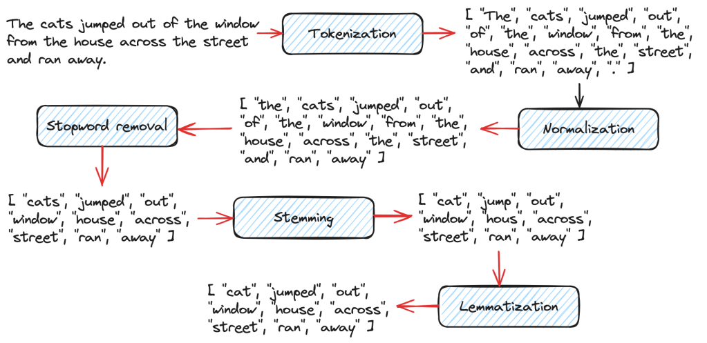
Indexing refers to storing data efficiently for fast retrieval at search time. Search Engines usually build an Inverted Index which maps terms to document IDs. The term frequency and the term positions are also stored along with the document ID. This list is commonly referred to as a Postings list.

Distributing data across multiple servers allows for scaling the cluster later as the data size increases. We need to load only a small part of the data into memory during search time. We can also employ techniques such as Scatter-Gather where the search requests are sent to multiple clusters/ shards in parallel which enables fast search operations.

Partitioning of indexes can be done in several ways:

ID Sharding – each shard contains a range of IDs and we try to maintain a relatively even distribution of data across the different shards.
Geo Sharding – each shard contains a range of documents from a certain geo location or region.
Hash-based Sharding – hash functions are applied to the sharding key to decide the shard to which the data is to be indexed. Hash collisions should be handled carefully.

We can also do Hybrid Sharding combining multiple sharding strategies based on the use case.

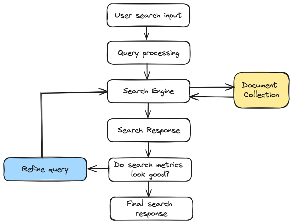
Distributed Search Operations

It is good design to have a set of coordinator nodes that take an incoming query and route it to the right node for searching. Coordinators can also send requests to multiple nodes in parallel, aggregate the results before sending a final response back to the user.

This type of parallel processing is one of the key advantages of a distributed search infrastructure.

To decide which results are the most accurate and relevant results to show to the user, search engines employ various algorithms that calculate the Precision and Recall scores before returning only the top results. Further manipulation and filtering can be done on top of these ranked results to make the results better.

There are two main types of Query Routing to do search operations:

Using Sharding – In this case, an algorithm will determine which shards the query needs to be sent to.
Scatter Gather – the query will be sent to all the nodes and the results will then be merged.

Evaluating the performance of a Distributed Search Infrastructure

We can look at a few key metrics that ensure that our Distributed Search Infrastructure is as efficient as possible and ensures the best user experience.

Indexing Speed

The speed at which data is indexed to the search infra and made available for users to search. Ensuring high indexing speeds means users are able to search on the latest data.

Search Latency

This is the time taken for the search query to execute and return a response to the user. This is key metric to ensure the best user experience.

Query Throughput

This measures the ability of the Search Infrastructure to handle a large volume of queries where many queries are made at the same time. So this is the number of queries processed per second.

Distributed Search Infrastructures form a crucial part of several websites and products that we use these days. I hope you enjoyed reading this short blog post on the its fundamentals. I will be back soon with another informative post!

Build a Simple Apache Lucene Search Application using Java Spring Boot

Posted on May 21, 2024November 11, 2024 by Swetha Kannan

In this tutorial, we are going to build a bare bones Search Application using Apache Lucene and Java Spring Boot. You will learn the basics of a Lucene Search Application by the time you finish this tutorial.

I have also attached the link to the full GitHub code in case you want to dive deeper into the code right away.

What is Apache Lucene?

Apache Lucene is a powerful Open Source Java library with Indexing and Search capabilities. There is also PyLucene with Python bindings for Lucene Core. Our tutorial will be in Java. Several Search Applications that are widely used in the industry today use Apache Lucene behind the scenes. This includes Elasticsearch, Nrtsearch, Cloudera, Github, Solr etc.

In this tutorial, you will learn to set up a simple Search Application using Apache Lucene in Java Spring Boot which is also an open source tool that makes setting up RESTful applications simple and easy.

Components of a Simple Search Application

Indexer

Inverted Index

Apache Lucene can perform fast full-text searches because of indexes that are built as Inverted Indexes. This is different from a regular index and for each term that appears in a pool of documents, the document ID and the position of that term in the document is stored. This list of doc IDs and positions is called a Postings List. The diagram below shows an example with only the doc IDs for each term. This allows fast look up during query time.

Lucene Indexer

The Lucene Indexer does a list of steps to convert raw text documents into Inverted Indexes. These include text analysis, splitting the text into smaller tokens and other processing such as stop words removal, lemmatization etc. There are several Analyzers available in Lucene based on user and language needs. In this tutorial, we will be using the Lucene StandardAnalyzer.

We will create a Lucene Document object which gets stored in Lucene Indexes from the raw text files. A Search Query in Lucene returns a set of Documents as the result. A Document contains a collection of Fields where each Field is a combination of Field name and a value that can be retrieved at search time using a Query.

In the code example below, we declare the path to the Index Directory. This is where the index files get stored. The Index Directory is a normal file system location on the local device and you will see it being created at the mentioned path once you run the indexing method. We initialize an IndexWriterConfig instance with a Lucene StandardAnalyzer and create an IndexWriter to index all the documents.

Directory indexDirectory = FSDirectory.open(Paths.get(INDEX_DIR));
IndexWriterConfig indexWriterConfig = new IndexWriterConfig(analyzer);
IndexWriter indexWriter = new IndexWriter(indexDirectory, indexWriterConfig);

// The file can be indexed using the IndexWriter as follows.
indexDocument(indexWriter, file);

// Method where the file contents get converted to a Lucene Document object before being indexed.
private void indexDocument(IndexWriter indexWriter, File file) throws IOException {
    Document doc = new Document();
    doc.add(new StoredField("fileName", file.getName()));
    doc.add(new TextField("fileContent", new FileReader(file)));
    indexWriter.addDocument(doc);
}

We map the indexing method to the path /index in our Spring Boot Application running on localhost:8080 which will produce the following output when indexing is done. Only 5 static files are used as Documents to keep things simpler. So this is a GET method in the code example.

Query

Query is the user-facing component of Lucene. A user can send any type of Lucene Query such as a BooleanQuery, TermQuery, PhraseQuery, PrefixQuery, PhraseQuery, FuzzyQuery etc. For our example, we are using a simple Lucene TermQuery.

A TermQuery consists of a field name and a value. Lucene will return the Documents that contain the specific term. The example below from the GET request that is sent to the search application contains the following components.

TermQuery – type of Query to map the Search Request to.
maxHits – the maximum number of documents to return for the result.
fieldName – the name of the Document Field
fieldValue – the specific Term to search for in the Lucene Documents.

body: JSON.stringify({
    "type": "TermQuery",
    "maxHits": 4,
    "fieldName": "fileContent",
    "fieldValue": "lucene"
})

We will convert the above Json Query into a Lucene TermQuery using a simple method as shown below.

public Query parseJsonToQuery() {
    return new org.apache.lucene.search.TermQuery(new Term(fieldName, fieldValue));

In this example, we want Lucene to return all Documents (maximum of 4) that contains the term “lucene” in the “fileContent” Field.

Searcher

Searching in Lucene is the process where a user Query is sent as a search request using the Lucene IndexSearcher. See below for the example.

IndexSearcher – used to search the single index that we created in the above step.
Query – the JSON request is parsed into a TermQuery in this case based on the specified type.
maxHits – the maximum number of Documents to return in the search response.
ScoreDoc[] – The indexSearcher.search() method returns a list of hits called TopDocs which are the Documents that satisfy the given Query. ScoreDoc contains the doc ID of the hit and the Relevance Score that was assigned by Lucene based on the match criteria of the Documents to the given Query.

@RequestMapping(
    value = "/search",
    method = RequestMethod.POST,
    produces = "application/json; charset=utf-8",
    consumes = MediaType.APPLICATION_JSON_VALUE)
public List<String> search(@RequestBody SearchRequest searchRequest) throws IOException {
    List<String> results = new ArrayList<>();

    Directory indexDirectory = FSDirectory.open(Paths.get(INDEX_DIR));
    IndexReader indexReader = DirectoryReader.open(indexDirectory);
    IndexSearcher indexSearcher = new IndexSearcher(indexReader);

    Query query = searchRequest.parseJsonToQuery();
    int maxHits = searchRequest.getMaxHits();

    ScoreDoc[] hits = indexSearcher.search(query, maxHits).scoreDocs;
    for (ScoreDoc hit : hits) {
      Document doc = indexSearcher.doc(hit.doc);
      results.add(doc.get("fileName"));
    }
    return results;
}

The /search POST request looks something like this.

fetch('http://localhost:8080/search', {
    method: 'POST',
    headers: {
        'Content-Type': 'application/json'
    },
    body: JSON.stringify({
        "type": "TermQuery",
        "maxHits": 4,
        "fieldName": "fileContent",
        "fieldValue": "lucene"
    })
})
.then(response => response.json())
.then(data => console.log(data))
.catch(error => console.error('Error:', error));

To send requests like this to our Spring Boot Application,

Go to localhost:8080 on the browser
Right click and choose Inspect
Go to Console, paste the above code and click Enter.

Alternatively, you can also send CURL requests from your terminal. Examples are linked in the readme document of the Github Repo.

You should see some results as shown below in the Console. Document 2, 5, 4 and 1 were the top ranked results by Lucene.

The full code can be found on my Github. I highly recommend that you take a look to understand this tutorial well. Feel free to download the project and add more capabilities to your Search Application. One idea is to add support for more types of Lucene Queries.

Hope you enjoyed reading this tutorial on setting up a Simple Lucene Search Application using Java Spring Boot. See you in the next blog post!

Search and Ranking

Introduction to Information Retrieval

Posted on February 21, 2024 by Swetha Kannan

Information Retrieval is the process of finding the most relevant information from a large collection of data (set of documents) for a given user query. Information Retrieval is the back bone of several systems such as

Web Search
Email Search
Library catalogs
ChatGPT etc

In this post, we will be learning about the following topics.

General Search Process
Document Indexing – Inverted Index
Text Processing
Types of Retrieval Models
Metrics to Evaluate Search

General Search Process

The following diagram gives an idea of the overall search process. When a user searches for a certain information, that information is transformed into a query that can be understood and processed by the search engine.

The query is then processed by the search engine to retrieve the most relevant documents from the collection. Certain metrics are used to evaluate the search response and if the results are not satisfactory, we refine the query further and reprocess it.

Document Indexing – Inverted Index

In order to retrieve information as fast as possible, we need to index the documents efficiently. We build what is called an “Inverted Index” for fast look up of documents that are most relevant to a search input.

An inverted index is a mapping of the different terms in a large collection to a list of documents in which the term occurs. The document is usually referred to by the document ID aka doc ID. The list of doc IDs is called a postings list. A variable length postings list is used to keep it updated as documents get updated.

Text Processing

Before building the inverted index, a number of text processing steps are performed on the documents in order to retrieve information effectively and minimize storing unnecessary words.

Tokenization

This step breaks down the given documents or text into individual words called tokens.

Normalization

At this step, extraneous details such as caps lock, punctuation etc are removed.

Remove Stopwords

There are many words such as “the”, “a” etc which don’t have any significance, so these are removed.

Stemming and Lemmatization

Stemming removes unwanted prefixes and suffixes from words. For ex: running -> run, books -> book.

Lemmatizers on the other hand, transform a word to its language-specific dictionary form. This produces more linguistically accurate words.

Types of Retrieval Models

Boolean Retrieval Model

This model can process Boolean queries that involve Boolean operators such as AND, OR, NOT etc. The inverted index is built based on the presence of terms in documents. This is simple and pretty popular but it cannot process queries that require contextual understanding.

Probabilistic Retrieval Model and BM25

This model ranks the documents based on the probability of their relevance to the search query. Okapi BM25 where BM stands for “Best Matching” is one of the most popular algorithms under the Probabilistic Retrieval Model. It calculates the document scores using various parameters such as term frequency, inverse document frequency, document length normalization etc.

Vector Space Model

In this model, data and queries are transformed into vectors in a multi-dimensional space. The number of dimensions will depend on the features used to represent the data. There are various distance metrics that can be used to compute the distance between points that capture semantic similarity but cosine distance is a popular one. This is a great model to capture contextual information.

Latent Semantic Indexing

This model captures latent semantic relationships between documents and terms using Singular Value Decomposition (SVD) to identify underlying concepts within a body of text. SVD is a technique to reduce dimensionality while preserving contextual information at the same time.

Neural Information Retrieval

NIR can capture complex semantics in text data thereby improving the accuracy and relevance of search. This model uses Neural Networks to retrieve highly relevant documents during search.

Metrics to Evaluate Search

There are two popular metrics to evaluate how good search results are. Although there are many others that we will be looking into in the future, these two are important.

Precision – This metric refers to the fraction of documents retrieved by search that are relevant to the user query. This points to the accuracy of the search results. Precision values are between 0 and 1 where 1 means a perfect accuracy score where all the documents were relevant to the search query.
Recall – This metric refers to the fraction of relevant documents retrieved by search from the total number of relevant documents in the collection. Recall values also range from 0 to 1 with 1 meaning that all the relevant documents in the collection were retrieved by the search operation.

Hope you enjoyed this Introduction to Information Retrieval post. Let us continue exploring various topics related to Information Retrieval and Semantic Search in future posts. Have a wonderful day!

AI/ Machine Learning, Search and Ranking, Software Engineering

K-Nearest Neighbors (KNN) Algorithm

Posted on February 12, 2024 by Swetha Kannan

We learnt about Semantic Search in my previous post. Here is the link if you missed it. K-Nearest Neighbors is one of the most popular Machine Learning algorithms used in semantic search to find documents or data that is semantically similar to a user’s query.

To recap, documents are represented as vector embeddings in a vector space model that captures semantic similarities based on the context. A user query is then converted to a vector embedding and efficient algorithms such as KNN, ANN (Approximate Nearest Neighbor) search are used to find the nearest neighbors to the query. This is where K-Nearest Neighbors algorithm is used where “K” refers to the number of nearest neighbors we want to consider before prediction.

How does KNN work?

KNN works by finding the “K” nearest neighbors in a vector space model. The value of K needs to be chosen carefully to balance between noise and over smoothing. One way is to test for accuracy of the algorithm by evaluating on different values of K using cross-validation where data is divided into training and validation datasets. The validation data set is used to evaluate the performance of the algorithm. A plot with K values and the corresponding error rate can help determine the best K value with the minimum error rate.

KNN finds the nearest neighbors using distance metrics. This can be anything such as Euclidean distance, Manhattan distance etc. We will look at the various distance metrics in detail in the next section.

KNN can be used for both Classification and Regression problems.

For Classification problems, the majority class is chosen among the K nearest neighbors.
For Regression problems, the average (or the weighted average) of the K nearest neighbors is used.

Distance Metrics

Various distance metrics are used for KNN, Euclidean distance being one of the most common ones.

Euclidean Distance

{\displaystyle d(p,q)={\sqrt {(p_{1}-q_{1})^{2}+(p_{2}-q_{2})^{2}+\cdots +(p_{n}-q_{n})^{2}}}.} — Source: Wikipedia

Euclidean Distance gives the straight line distance between two coordinates in a vector space. This works great for numerical features in the input data.

Manhattan Distance

{\displaystyle \sum _{i=1}^{n}|p_{i}-q_{i}|} — Source: Wikipedia

Manhattan Distance calculates the sum of absolute differences between the vector data points. This is good with categorical features. It is not as sensitive to outliers as Euclidean Distance.

Mikowski Distance

{\displaystyle D\left(X,Y\right)={\biggl (}\sum _{i=1}^{n}|x_{i}-y_{i}|^{p}{\biggr )}^{\frac {1}{p}}.} — Source: Wikipedia

Mikowski Distance is a generalization of the above distances.

If p = 1, we get Manhattan Distance
If p = 2, we get Euclidean Distance

Hamming Distance

Hamming Distance between two vectors of same length is the number of positions where the corresponding vector values are different. This is suitable for categorical and even binary data.

Cosine Similarity

This is commonly used for high dimensional vector data or text data and it calculates the distance using the cosine of the angle between two vectors.

KNN Algorithm Example for Classification

We have a good understanding of KNN. Now let us look at an actual code example of KNN for a Classification problem.

As a coding exercise, try to implement the averaging functionality for a regression KNN algorithm on your own.

from algorithms.knn import distances

METRICS = {
    "euclidean": distances.EuclideanDistance(),
    "manhattan": distances.ManhattanDistance(),
    "mikowski": distances.MikowskiDistance(),
    "hamming": distances.HammingDistance(),
    "jaccard": distances.JaccardDistance(),
    "cosine": distances.CosineDistance()
}


def get_majority_element(computed_distances):
    """
    Takes an iterable of tuples (distance, class_type)
    and finds the majority class_type
    :param computed_distances: iterable of tuples
    :return: majority element: string
    """
    freq = {}
    for _, class_type in computed_distances:
        if class_type not in freq:
            freq[class_type] = 1
        else:
            freq[class_type] += 1
    return max(freq, key=freq.get)


def knn(training_data, k, distance_metric, test_value):
    """
    Find the k nearest neighbors in training_data for the
    given test value to determine the class type
    :param training_data: Dictionary of class type keys and list of vectors
    as values
    :param k: Integer
    :param distance_metric: string
    :param test_value: query vector
    :return:
    """

    if distance_metric not in METRICS:
        raise ValueError(distance_metric + "is not a valid input")

    distance_calculator = METRICS[distance_metric]
    computed_distances = []

    for class_type, points in training_data.items():
       for point in points:
           distance = distance_calculator.calculate(point, test_value)
           computed_distances.append((distance, class_type))

    # sort the tuples by the computed distance
    computed_distances.sort()
    return get_majority_element(computed_distances[:k])

from abc import abstractmethod, ABC
from math import pow, sqrt

ROUND_TO_DECIMAL_DIGITS = 4

class Distances(ABC):
    @abstractmethod
    def calculate(self, x1, x2):
        pass

class EuclideanDistance(Distances):
    def calculate(self, x1, x2):
        """
        Compute the Euclidean distance between two points.

        Parameters:
        x1 (iterable): First set of coordinates.
        x2 (iterable): Second set of coordinates.

        Returns:
        float: Euclidean Distance
        """
        if len(x1) != len(x2):
            raise TypeError("The dimensions of two iterables x1 and x2 should match")
        return round(sqrt(sum(pow(p1 - p2, 2) for p1, p2 in zip(x1, x2))), ROUND_TO_DECIMAL_DIGITS)

Real World Applications of KNN

KNN is used in a variety of applications such as

Recommendation Systems – to recommend the most popular choices among users for collaborative filtering by identifying users with similar behavior.
Disease Classification – it can predict the likelihood of certain conditions using majority voting.
Semantic Search – to find semantically similar documents or items for a user’s query.
Text Classification – spam detection is a good example.
Anomaly Detection – It can signify data points that differ from the rest of the data in a system and many many more.

I hope you enjoyed reading about K-Nearest Neighbors algorithm. We will continue to explore various topics related to Semantic Search as well as Search and Ranking in general over the next few weeks.

If you like learning about these types of concepts, don’t forget to subscribe to my blog below to get notified right away when there is a new post 🙂 Have an amazing week ahead!

Search and Ranking

Introduction to Semantic Search

Posted on February 5, 2024 by Swetha Kannan

Semantic search is a type of search that takes into account the meaning and context of a query from a user as opposed to lexical search which only looks for exact keyword match of the query terms.

As an example, when a user searches for the term “football”, we want the search to also consider words such as “soccer”. When “football” is misspelled as “ftball”, we still want to match with “football”.

Semantic search has the ability to dramatically improve the user experience by improving the quality of search results. This is achieved by various Machine Learning models and AI technologies.

Structured Vs Unstructured Data

Structured data is well-defined and is easily searchable whereas unstructured data can be anything such as photos, audio, videos, paragraphs of texts, emails etc and is harder to search through.

Structured data fits well into a storage solution such as a relational database and is searchable using SQL queries but unstructured data does not and needs to be processed using machine learning algorithms to get relevant search results.

As much as 80% of data out there is unstructured. This is important for semantic search because it works on unstructured data which needs to be indexed in a way that it is searchable as efficiently as possible.

Transforming Unstructured Data Using Vector Embeddings

In order for Machine Learning algorithms to process unstructured data to get the most relevant results, this data needs to be represented in a way that the ML models can understand.

This is where Vector Embeddings become useful. Vector Embeddings represent data in numerical form. This opens up a world of computational possibilities on this data. Vector Embeddings transform unstructured data into points in the vector space where similar points get clustered together. This means words, sentences, audio data etc can be represented as vectors which get clustered together in an n-dimension vector space according to their similarity. This is then used by machine learning algorithms to find patterns using which we can do queries that find the most relevant search results.

Here is an example of a 5 dimensional vector embedding. Each point in the vector refers to a feature representing the data.

[1.0, 3.0, 5.0, 7.0, 9.0]

There are various types of embeddings such as word embeddings, graph embeddings, image embeddings etc. The most common type of embeddings used are word embeddings which is used to represent textual data and is used in Semantic Search.

Indexing Vector Data

When data is represented as vector embeddings, it can have high dimensionality based on the number of features used to represent the data. We therefore need a way to efficiently search through large sets of vector embeddings.

Indexing the vector data in the right way helps in efficiently retrieving the most relevant results during search. There are various indexing algorithms proposed for this but a couple of them are highly popular.

Locality Sensitive Hashing (LSH)

This technique is used to do an approximate nearest neighbor search in high dimension vector space. LSH is a hashing based algorithm that will hash similar points to the same or nearby buckets with a high probability so that the search space reduces. Collisions are maximized for similar inputs unlike traditional hashing where we minimize them. This makes it faster to find the approximate nearest neighbors.

Some parameters that need tuning to achieve a good trade off between accuracy and efficiency are hash size, number of hashing functions, number of hash tables etc.

Hierarchical Navigable Small Worlds (HNSW)

HNSW is a graph based data structure that can be used for approximate nearest neighbor search. This works great for high dimensionality vector data since it navigates the graph efficiently for similarity search.

The graph data structure is organized into levels with the bottom layer containing the most data points and each layer above it being a subset of the previous one. The vertices are created such that the likelihood of a graph node appearing in top layers decreases exponentially, which helps keep the graph sparse at higher levels enabling efficient search.

During a search operation, we start at the top most layer and navigate towards the bottom of the graph to find the nearest neighbors that decrease the distance to the input data points. This means we are searching more coarsely at the top instead of having to search the entire graph and keep refining the search as we get to the bottom layer.

In the example above, we want to find the nearest neighbor of the red dot. So we start at the top most layer at an entry point node and traverse to the neighbor, we then go to the next levels to try and find the nearest neighbor. This is an oversimplification of HNSW works but we will look at this topic in detail on another post.

HNSW are efficient and have good accuracy, thereby being the most popular algorithm for vector similarity search at the moment. HNSW may not suit data that gets frequent updates since reconstructing the graph often is an expensive process.

Searching on Vector Data

Vector search also known as nearest neighbor search is what powers several semantic search use cases. This works efficiently on vector embeddings that we learnt about in the previous section. Since the search query is also represented as a vector, finding the most relevant results would mean searching for the nearest neighbors for the given query data.

The most popular algorithm for doing a nearest neighbor search in kNN – k nearest neighbor search. This provides highly accurate results but it is also computationally intensive. For large language model datasets, this does not scale well. So in these cases, the ANN – Approximate Nearest Neighbor search works much better at the cost of slightly reduced accuracy. We will learn about KNNs and ANNs in future posts on this topic.

Hope you enjoyed learning about semantic search. Let’s continue to explore this topic in more detail.