Swetha Kannan

Search in a Binary Search Tree

Posted on July 10, 2020July 10, 2020 by Swetha Kannan

We are given the root of a BST and a target value to search for. If the target node exists, return the subtree rooted at that node, else return NULL.

Example: Value to search for = 2

Output:

      2     
     / \   
    1   3

Solution:

Binary Search Trees (BST) have this incredible property where an inorder traversal yields nodes in sorted order. This is because each node’s value is greater than all the values in its left subtree and lesser than all the values in its right subtree.

Armed with this knowledge, what we essentially do is to search for the given value in a sorted list. What is the most efficient way to search in a sorted list? Yes, binary search, where at each step we try to cut down our search space by half. In the case of a BST, this equals eliminating either the left or the right subtree of a node from our search space. Now this works well in a balanced BST where the number of nodes in the left and right subtrees are fairly equal. When the tree is skewed to the left or to the right, it’s the same as doing a linear search.

Our search algorithm is as follows:

Start at the root node. If the root = target, return root.
If root < target, then the target might be in the right subtree. We then recursively search the right subtree only.
If root > target, then the target might be in the left subtree. We then recursively search the left subtree only.
If the value wasn’t found, return NULL.

Time Complexity: O(log N) in a balanced BST but O(N) in a skewed tree where N is the number of nodes in the tree.

Space Complexity: O(log N) for the use of recursive stack space. O(N) at the worst case when the tree is skewed.

Code:

def searchBST(self, root: TreeNode, val: int) -> TreeNode:
    def searchHelper(root, val):
        if not root:
            return None
        if root.val == val:
            return root
        if root.val < val:
            return searchHelper(root.right, val)
        else:
            return searchHelper(root.left, val)
    return searchHelper(root, val)

Hope you enjoyed this simple but delightful problem! Have a nice day!

Data Structures/ Leetcode, Graphs, June Leetcoding Challenge

Find cheapest flights within K stops

Posted on July 8, 2020July 9, 2020 by Swetha Kannan

There are n cities connected by m flights. We are also given a list with elements containing three pieces of information [u, v, w] where:

Source city: u
Destination city: v
Price to fly from u to v: w

Our goal is to find the cheapest flight ticket from a given source city src to a destination city dst with up to k stops. If no route exists, return -1.

Example 1:
Input:
n = 3, edges = [[0,1,100],[1,2,100],[0,2,500]]
src = 0, dst = 2, k = 1
Output: 200
Explanation:
The graph looks like this:

The cheapest price from city 0 to city 2 with at most 1 stop costs 200, as marked red in the picture.

Solution:

This problem can be re-phrased as trying to find the shortest path between nodes in a weighted graph. Here the nodes are the cities and the weights refer to the flight prices. The simplest graph algorithm to find the shortest path in a weighted graph is Dijkstra’s Shortest Path First algorithm. If this was an unweighted graph, Breadth First Search would have been our ideal choice. This is a good difference to remember. In interviews, the first right move is to model the problem correctly. The next move is to narrow down to the right choice of algorithms.

To solve a graph problem, we have to first construct the graph from the edges. In this problem, for every source city, we store information about the destination cities that we can get to, as well as the corresponding prices. Our constructed graph will look like this.

edges = [[0, 1, 100], [1, 2, 100], [0, 2, 500]]

0: [(1, 100), (2, 500)]
1: [(2, 100)]

How can we make sure to always pick the path with the lowest weight? What kind of data structure always yields the lowest value? If you haven’t guessed it yet, the answer is a min-heap/ priority queue.

The only catch in this problem is the added restriction of having to reach our destination in at most K stops. Therefore, our priority queue contains elements that hold three key pieces of information.

The current node src
The lowest cost to current node
Minimum number of stops to get to the current node

Note that the priority queue will always give us the element with the lowest cost. We will process the queue as long as there are elements left in it or until we reach the destination dst node. This will be our algorithm at each iteration.

Pop the lowest cost element from priority queue. This gives us three values curr_node, curr_cost, curr_stops.
If the curr_node is the same as the destination dst node, return the curr_cost where curr_cost gives the lowest cost with at most K stops to get to the destination.
If the curr_node is not the destination and curr_stops <= K, then we iterate through the edges of this node stored in our graph. Note that each graph vertex may have multiple routes/ edges to different cities.
A neighboring edge contains a vertex v and cost c to get there. We will push (v, cost, K) to the priority queue where cost and K are obtained as follows.
- cost = curr_cost + c
- K = curr_stops + 1

Look at the picture below that walks you through the given example step by step.

Time Complexity: The complexity is defined by the number of pop operations we have to do with the min-heap and the number of edges we process for each graph node. Popping from heap takes logarithmic time, so ignoring duplications in the heap, time complexity will be log V. The graph we constructed is an adjacency matrix representation, so the worst case complexity will be V². The overall complexity is O(V² log V). Note that the heap complexity will be more than log V since we add the same node to the heap more than once to find the shortest path with K stops.

Space Complexity: O(V²) referring to the maximum space taken up by the adjacency matrix. Conservatively, the heap takes O(V) space.

Code:

def findCheapestPrice(self, n: int, flights: List[List[int]], src: int, dst: int, K: int) -> int:

        graph = collections.defaultdict(list)

        for s, d, c in flights:
            graph[s].append((d, c))

        pq = [(0, src, 0)] 

        while pq:
            curr_cost, curr_node, curr_stops = heapq.heappop(pq)

            if curr_node == dst:
                return curr_cost

            if curr_stops <= K:
                for dest, cost in graph[curr_node]:
                    heapq.heappush(pq, (curr_cost + cost, dest, curr_stops+1))

        return -1

Hope you enjoyed reading the solution to this problem 🙂 Have a great day!

Arrays and Strings, Data Structures/ Leetcode, June Leetcoding Challenge

Largest Divisible Subset

Posted on June 27, 2020June 27, 2020 by Swetha Kannan

Given a set of distinct positive integers, find the largest subset such that every pair (Si, Sj) of elements in this subset satisfies:

Si % Sj = 0 or Sj % Si = 0

If there are multiple solutions, returning any subset is fine.

Example 1:

Input: [1,2,3]
Output: [1,2] or [1,3]

Example 2:

Input: [1,2,4,8]
Output: [1,2,4,8]

Solution #1:

Let’s say we have a list of numbers as shown below.

nums = [1, 2, 3, 4]

First thing to notice is that every integer is its own largest divisible subset if the given condition does not satisfy for any other element in the list. For example, given a list [5, 7] where neither of them are divisible by each other, the largest divisible subset can be [5] or [7], so both are correct.

Keeping that in mind, a straightforward approach is to check every integer with every other integer in the list to see if the condition Si % Sj = 0 or Sj % Si = 0 is satisfied. Before we begin, we sort the given list so that we can avoid having too many enumerations. Let’s understand this using another example as shown below.

[2, 4, 8]

Note that the list above is sorted in ascending order and all the elements form a divisible subset. If we choose to add one more element d to the divisible subset at front or an element D at the end of the list, all we have to check is whether D % 8 == 0 and 2 % d == 0.

At first we place each integer in its own subset. Then, we can iterate through the list using double for loops and whenever a pair satisfies the given condition, we extend the individual subsets. We start with the following subsets.

[{1}, {2}, {3}, {4}]

Use two pointers i and j where i is used to traverse the sorted list [1, 2, 3, 4]
Calculate the largest divisible subset that ends at the element at i. Use another pointer j to traverse the list until the index i.
If the values at i and j satisfy the divisibility condition ie. nums[i] % nums[j] == 0 and if the (size of the subset at i) < (size of subset at j + 1), then extend the subset at i. This is because we want to extend the subset only if we can get another larger subset, otherwise it’s already the largest subset possible ending with element at i.

To understand clearly, check the example walkthrough below.

Once we have all the subsets, we return the one with the max length.

Time Complexity: O(N²) since we use double for loops

Space Complexity: O(N²) for the use of subsets

Code:

def largestDivisibleSubset(self, nums: List[int]) -> List[int]:

    if not nums:
        return []

    nums.sort()
    subsets = [{i} for i in nums]

    for i in range(len(nums)):
        for j in range(i):
            if nums[i] % nums[j] == 0 and len(subsets[i]) < len(subsets[j]) + 1:
                subsets[i] = subsets[j] | {nums[i]}

    return max(subsets, key = len)

Hope you enjoyed learning how to solve the largest divisible subset problem. Have a great day!

Arrays and Strings, Design Coding Problems, Hashmaps, June Leetcoding Challenge

Insert Delete and Get Random in O(1)

Posted on June 20, 2020June 21, 2020 by Swetha Kannan

Today, we will be discussing one of my favorite problems because it’s open ended and design oriented. We have to design a data structure that can perform insert, delete and get random operations with an average of O(1) time complexity.

insert(val): Inserts an item val to the set if not already present.
remove(val): Removes an item val from the set if present.
getRandom: Returns a random element from current set of elements. Each element must have the same probability of being returned.

Let’s take a look at our toolbox to see what data structures we can use in solving this problem. The table below lists the average time complexity for some of the operations.

Data structure	Access	Insert	Delete
Arrays	O(1)	O(N)	O(N)
Stacks	O(N)	O(1)	O(1)
Queues	O(N)	O(1)	O(1)
Hashmap	O(1)	O(1)	O(1)
Linked List	O(N)	O(1)	O(1)

Average time complexity

The above table shows that most of the data structures except arrays have an average time complexity of O(1) to perform insert and delete operations but remember that inserting and deleting from the end of an array is still O(1). The catch here is to get the getRandom function perform at O(1) time. We cannot get a random index from Hashmaps and accessing indexes takes O(N) time with other data structures except for arrays. In this case, we can leverage the benefits of hashmaps and arrays by doing the following.

Insertion O(1)

Insert an element at the end of an array
Store the insertion indexes of elements in a hashmap

Remove O(1)

Find the index of the element to be removed, from the hashmap
Copy the last element of the array into this index
Pop the last element of the array O(1)
Delete the entry for this element from the hashmap

Get Random O(1)

Use a random function to get an index between 0 and len(array) – 1
Return the element at that index from the array

Time Complexity: All operations happen in O(1)

Space Complexity: O(N) for the array and O(N) for the hashmap, so the overall space complexity is O(N)

Code:

class RandomizedSet:
    def __init__(self):
        """
        Initialize your data structure here.
        """
        self.nums = []
        self.mapping = {}
        
    def insert(self, val: int) -> bool:
        """
        Inserts a value to the set. Returns true if the set did not already contain the specified element.
        """
        if val not in self.mapping:
            # Insert the element at the end of nums
            self.nums.append(val)
            index = len(self.nums) - 1
            self.mapping[val] = index
            return True
        return False
    
        
    def remove(self, val: int) -> bool:
        """
        Removes a value from the set. Returns true if the set contained the specified element.
        """
        if val not in self.mapping:
            return False
        
        removeIndex = self.mapping[val]
        lastValue = self.nums[-1]
        # store the last element in the removed val index
        self.nums[removeIndex] = lastValue
        # Update the index value of last element
        self.mapping[lastValue] = removeIndex
        # clean up
        self.nums.pop()
        del self.mapping[val]
        return True
        
    def getRandom(self) -> int:
        """
        Get a random element from the set.
        """
        randIndex = random.randint(0, len(self.nums) - 1)
        
        return self.nums[randIndex]
# Your RandomizedSet object will be instantiated and called as such:
# obj = RandomizedSet()
# param_1 = obj.insert(val)
# param_2 = obj.remove(val)
# param_3 = obj.getRandom()

Hope you enjoyed learning how to design a data structure that can perform insert, delete and get random operations in O(1) time. Have a great day!

Arrays and Strings, June Leetcoding Challenge, Two Pointer Technique

[Problem Solving] Sort Colors – Variation of Dutch National Flag Problem

Posted on June 18, 2020June 23, 2024 by Swetha Kannan

Given an array containing integers 0, 1 and 2 representing the colors red, white and blue, sort them in-place so that the same numbers are adjacent, with the order being 0, 1 and 2.

Example:

Input: [2,0,2,1,1,0]
Output: [0,0,1,1,2,2]

Solution #1:

There are only three different values in the array and those are 0, 1 and 2. We have to return an array arranged in an order with all the numbers with same values clubbed together. A simple approach is to count the number of 0s, 1s and 2s in the given array and overwrite the given array with these three values according to the counts. In the given array,

count(0) = 2

count(1) = 2

count(2) = 2

So let’s say we store these values in an array counts = [[0, 2], [1, 2], [2, 2]]. We can then iterate through this array and overwrite the given input array with 0, 1 and 2 according to their respective counts.

Time Complexity: O(N) to count the values and another O(N) to overwrite the input array, so the overall time complexity will be O(N).

Space Complexity: O(C) since we use constant space to store the values 0, 1, 2 and their counts.

Solution #2:

Notice that we have to shuffle around only three different values. This means that we can use a few pointers to keep track of some of the values.

Let’s use three different pointers as follows.

zero_ptr to keep track of the leftmost index where we can overwrite with a 0.
two_ptr to keep track of the rightmost index where we can overwrite with a 2.
curr pointer to keep track of the current index we are looking at.

Algorithm to get the Dutch National Flag pattern:

When curr points to a 0, we swap it with the element at zero_ptr. After swapping we move curr and zero_ptr one step forward.
When curr points to a 2, we swap it with the element at two_ptr. We then decrement the value of two_ptr. Note that we should not move curr at this step because we may have just swapped a 2 with another 2 and we should re-process it in the next step.
If curr points to a 1, we just move curr to the next element.

The above loop stops when curr > two_ptr. This indicates that we have placed all the values in their appropriate slots. If this is too confusing, look at the picture below to see how the algorithm works step by step.

Time Complexity: O(N)

Space Complexity: O(1) for in-place re-arrangement

Code:

def sortColors(self, nums: List[int]) -> None:
    """
    Do not return anything, modify nums in-place instead.
    """

    zero_ptr = curr = 0
    two_ptr = len(nums) - 1

    while curr <= two_ptr:
        if nums[curr] == 0:
            nums[curr], nums[zero_ptr] = nums[zero_ptr], nums[curr]
            zero_ptr += 1
            curr += 1
        elif nums[curr] == 2:
            nums[curr], nums[two_ptr] = nums[two_ptr], nums[curr]
            two_ptr -= 1
        else:  
            curr += 1

Hope you learnt how to solve this fun problem. Have a great day!

Arrays and Strings, Binary Search, June Leetcoding Challenge

Binary Search variations that you should know

Posted on June 15, 2020 by Swetha Kannan

Binary Search is a useful algorithm to search for a target value in a sorted list of elements.

Standard Binary Search:

Get the middle element of the sorted list and compare with the target value. If the number equals the target, we found the value.
If the middle element is less than the target, then we have to search in the right half of the sorted array.
Else we search in the left half of the sorted array.

Let us look at the code for standard Binary Search.

def binarySearch(self, nums: List[int], target: int) -> int:

    left = 0
    right = len(nums) - 1

    while left <= right:
        mid = (left + right) // 2

        if nums[mid] == target:
            return mid

        # search in the right half       
        if nums[mid] < target:
            left = mid + 1

        # search in the left half      
        else:
            right = mid - 1

    return -1

At each iteration of the while loop, the above algorithm divides our search space by half, so the overall time complexity will be O(log N). This is a significant reduction compared to the O(N) time complexity incurred by Linear Search. Now let’s look at a variation.

Binary Search Variation #1:

Given a sorted array and a target value, return the index if the target is found. If not, return the index where it would be if it were inserted in order.

Assumption: There are no duplicates in the array.

In this case, if a target is not found, we have to find the index of the value immediately greater than the target. Let’s look at an example.

Input: nums = [1,3,5,6], target = 4

Output: 2

In the above example, 4 is not present in the array. If we were to insert it into the array, we should insert it between 3 and 5. So our insert index will be 2.

We can use the standard binary search to find the insert position with a slight variation. Let’s run through the algorithm step by step.

left = 0, right = 3
mid = (0 + 3) // 2 = 1
nums[mid] = nums[1] = 3
Here 3 < 4, if nums[mid] < target, search the right half of the list
Then left = mid + 1 => 1 + 1 = 2

left = 2, right = 3
mid = (2 + 3) // 2 = 2
nums[mid] = nums[2] = 5
Here 5 > 4, if nums[mid] > target, search the left half of the list
Then right = mid -1 => 2 – 1 = 1

In the above example, we see that the left pointer holds the insert position as we go through the while loop. This is because, by the time we complete the while loop, left pointer will point to the element that is immediately greater than the target value which is where we will insert our target.

Code:

def searchInsert(self, nums: List[int], target: int) -> int:

    left = 0
    right = len(nums) - 1

    while left <= right:
        mid = (left + right) // 2

        if nums[mid] == target:
            return mid

        if nums[mid] < target:
            left = mid + 1

        else:
            right = mid - 1

    return left

Binary Search Variation #2:

Now what if we have to find the index of the element that is just smaller than the given target ie., the greatest element lesser than the target value. Yes, you guessed it! This value is stored by the right pointer, so we return it in that case.

Code:

def searchLesserThanTarget(self, nums: List[int], target: int) -> int:

    left = 0
    right = len(nums) - 1

    while left <= right:
        mid = (left + right) // 2

        if nums[mid] == target:
            return mid

        if nums[mid] < target:
            left = mid + 1

        else:
            right = mid - 1

    return right

Hope you enjoyed learning the different variations of Binary Search. Have a great day!

Arrays and Strings, Data Structures/ Leetcode, June Leetcoding Challenge, Two Pointer Technique

[Problem Solving] Is Subsequence – Two Pointer Technique

Posted on June 14, 2020June 23, 2024 by Swetha Kannan

Given two strings s and t, check if s is a subsequence of t. A subsequence can be formed by deleting some characters in a string without changing the order of the other characters.

Input: s = “abc”, t = “ahbgdc“
Output: true

The simplest way to solve this problem is to use the two-pointer technique where we designate two different pointers to traverse s and t simultaneously. If the characters match, then we move on to check the next character of s against t, otherwise we move on to the next character in t. By the time we are done, there should be no characters left in s to be compared and therefore s must be a substring of t.

Time Complexity: The loop ends when we run out of characters to compare in either s or t. The worst case happens when we run through all the characters in t, so the time complexity is O(T).

Space Complexity: O(1)

Code:

def isSubsequence(self, s: str, t: str) -> bool:

    i, j = 0, 0

    while i < len(s) and j < len(t):
        
        if s[i] == t[j]:
            i += 1
            
        j += 1
    return i == len(s)

Testing:

For this problem, the following test cases will cover various situations.

Empty s
Empty t
s string length greater than t
A few other random test cases

I find all other approaches to be kind of an overkill, so I hope you enjoyed this simple approach. Have a great day!

Bit Manipulation, Data Structures/ Leetcode, June Leetcoding Challenge

Where can you use the expression n & (n – 1) ?

Posted on June 12, 2020June 12, 2020 by Swetha Kannan

n & (n -1) is a pretty powerful bitwise operation and we will see why in this post.

Power of two

Given an integer, we have to write a function to determine if it is a power of two.

Examples:

Input: 1
Output: true
Explanation: 2⁰ = 1

Input: 32
Output: true
Explanation: 2⁵ = 32

Input: 100
Output: false

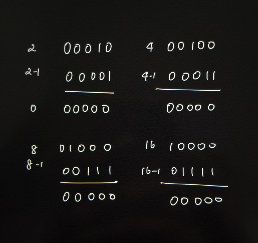
What do powers of two look like in binary representation?

1 – 1
2 – 10
4 – 100
16 – 1000
32 – 10000

Notice that the integers above have only one 1-bit followed by all zeroes.

When we subtract 1 from any number, the rightmost 1-bit gets set to 0 and all the bits following this rightmost 1-bit will be set to 1. Let’s look at a few examples. In binary subtraction, when we perform 0 – 1, the result is 1 with a borrow of 1 from the next higher order bit. Borrowing can be tricky, here is good video that goes over binary subtraction.

When we AND the results above with the original integers, the result is 0. To conclude, if n & (n – 1) equals zero, then the given integer is a power of two. Other numbers have more than one 1-bit in the binary representation, so this trick will not return zero for those cases.

Time Complexity: O(1)

Space Complexity: O(1)

Code:

def isPowerOfTwo(self, n: int) -> bool:

    if n == 0:
        return False
    return n & (n-1) == 0

Count the number of ones in an unsigned integer

Essentially what n & (n-1) does is that it sets the right most 1-bit in an integer to 0. If we do that repeatedly, at some point all the bits get set to 0. We can use this same expression to count the number of one bits in any given unsigned integer without having to count the ones by traversing bit by bit. The number of 1-bits in an integer is also known as the hamming weight of a number.

Time Complexity: An unsigned integer will be 4 bytes ie., 32 bits long at maximum. The worst case happens when all the bits of an integer are 1 and we have to loop through it 32 times setting the rightmost bits to 0. If we consider this to be a constant time operation since an integer can never have more than 32 bits, then the time complexity will be O(1).

Space Complexity: O(1)

Code:

def hammingWeight(self, n: int) -> int:

    count = 0

    while n:
        n &= n-1
        count += 1

    return count

Hope you had fun learning this useful bit manipulation trick. Have a nice day!

Data Structures/ Leetcode, Dynamic Programming, June Leetcoding Challenge

Coin Change – Dynamic Programming

Posted on June 8, 2020June 8, 2020 by Swetha Kannan

We are given an infinite supply of coins of ‘n’ different denominations and a total amount T. We have to find the total number of distinct ways in which we can make up this amount.

Input: amount = 5, coins = [1, 2, 5]
Output: 4
Explanation: There are four ways to make up the amount 5.
5=5
5=2+2+1
5=2+1+1+1
5=1+1+1+1+1

Infinite supply of coins means that we can choose the same coin multiple times in order to make up the total amount 5.

Solution #1: Let’s start with a brute force approach which is to try all the possible combinations from the given coins. Each combination is a subset of coins. For each coin, we can make two different decisions.

If the coin amount does not exceed the total give amount, we can INCLUDE THE COIN in our subset combination and then recursively make a decision on the remaining coins including the current coin, since we can repeatedly choose the same coin to get T.
Another option is to EXCLUDE THE COIN and create a new subset combination with the remaining coins.

The above points make up the core algorithm of this problem. Let’s say the total amount is T and C is the current denomination of the coin that we are processing. Then,

If we include the first coin C, the sum left to make up to T will be T – C and we process the list coins[0…n-1] since we are allowed to select the same coin again.
If we exclude the first coin, the sum left to make up to T will remain the same and we will process the list coins[1…n-1].

This gives way to a recursion tree as shown below.

Time Complexity: This algorithm has exponential time complexity O(2^C+T) where C is the total coins we are given and T is the total amount. This is because for each coin c and amount t, we have to make two decisions ie., branch into two recursive sub-problems of including and excluding the coin.

Space Complexity: O(2^C+T) since the recursion will use stack space that is as deep as the recursion tree.

Code for solution #1:

def change(self, amount: int, coins: List[int]) -> int:
    
    def countHelper(coins, totalAmount, coinIndex):
        
        # If the amount is 0, there is only one way to make this
        # Just exclude the coin
        if totalAmount == 0:
            return 1
        
        n = len(coins)
        # No coins left or all coins have been processed
        if n == 0 or currentIndex >= n:
            return 0
        
        includeCoinSum = 0
        if coins[coinIndex] <= totalAmount:
            includeSum = countHelper(coins, totalAmount - coins[coinIndex], coinIndex)
            
        excludeCoinSum = countHelper(coins, totalAmount, coinIndex + 1)
        
        return includeCoinSum + excludeCoinSum
    
    return countHelper(coins, amount, 0)

Solution #2: It’s pretty clear that an exponential algorithm is not efficient. This is when dynamic programming comes into action. Why is this problem a good candidate for dynamic programming?

Overlapping sub-problems: As we branch down the tree, we saw in the recursion tree image that we compute the total number of ways for some coin c and amount t repeatedly. If the tree size grows, the repetitions will be even higher. This means we can cache the results of a sub-problem and then re-use it the next time we want to compute the same. This is called memoization technique.

Optimal sub-structure: In any given problem, if we are able to compute the optimal solution for a larger problem by computing the optimal results for its smaller sub-problems, then it follows the optimal sub-structure property.

How can we choose what to memoize? To figure this part out, we look at the two variables that are constantly changing state in solution #1 code. This is the coinIndex and the totalAmount values which keep changing during every recursive call. So we store the count value (number of ways) to make an amount totalAmount with the coin at coinIndex during each recursive call. Our memoization array is a 2D array dp[len(coins)][totalAmount + 1] and the number of sub-problems that we need to solve will be C * T ie., for each grid in the 2D array.

Time Complexity: O(C * T) to compute all the sub-problems.

Space Complexity: O(C * T) for the dp array and the recursion costs another O(C) stack space, which adds up to O(C * T + C). So the overall space complexity will be O(C * T).

Code for solution #2:

def change(self, amount: int, coins: List[int]) -> int:
    
    def countHelper(dp, coins, totalAmount, coinIndex):
        
        # If the amount is 0, there is only one way to make this
        # Just exclude the coin
        if totalAmount == 0:
            return 1
        
        n = len(coins)
        # No coins left or all coins have been processed
        if n == 0 or currentIndex >= n:
            return 0
        
        if dp[coinIndex][totalAmount] != -1:
            return dp[coinIndex][totalAmount]
        
        includeCoinSum = 0
        if coins[coinIndex] <= totalAmount:
            includeSum = countHelper(dp, coins, totalAmount - coins[coinIndex], coinIndex)
            
        excludeCoinSum = countHelper(dp, coins, totalAmount, coinIndex + 1)
        
        dp[coinIndex][totalAmount] = includeCoinSum + excludeCoinSum
        return dp[coinIndex][totalAmount]
    
    dp = [[-1 for _ in range(amount+1)] for _ in range(len(coins))]
    
    return countHelper(dp, coins, amount, 0)

The above approach is called top down dynamic programming. This is because we start with the larger problem and recursively break it down into smaller sub-problems and compute their results. We can avoid recursion by approaching this problem bottom-up. In this case, we compute the results of sub-problems before using them to compute the larger problem. This method is called tabulation.

Solution #3:

We can use the same 2D array dp[len(coins)][totalAmount + 1] to populate the sub-problem results but this time we start from the smallest sub-problem. For this to make sense, we need to understand what a single sub-problem in this array means. dp[c][t] means the total number of ways to make up an amount t by including or excluding the coin at index c.

When we exclude a coin at index c, we can make a total t using dp[c – 1][t] number of ways. We use the coins up until the index c – 1 to make the amount t but we skip the coin at c.
When we include the coin at index c, we have to subtract its value from the total amount t ie., dp[c][t – coins[c]]

Adding the above two results gives the result for dp[c][t] ie. the total number of ways to make t using the coins up until index c.

dp[c][t] = dp[c – 1][t] + dp[c][t – coins[c]]

The dp array contains the following values for the given problem. Our answer is in the bottom right grid of the dp array when we compute dp[C][T] using all the sub-problems.

Time Complexity: O(C * T) to populate the dp array.

Space Complexity: O(C * T) for the 2D array.

Code for the above solution:

def change(self, amount: int, coins: List[int]) -> int:

    if not amount:
        return 1

    if not coins:
        return 0

    n = len(coins)
    dp = [[0 for i in range(amount+1)] for _ in range(n)]

    for i in range(n):
        dp[i][0] = 1

    for c in range(n):
        for t in range(1, amount+1):
            dp[c][t] = dp[c-1][t]

            if coins[c] <= t:
                dp[c][t] += dp[c][t - coins[c]]

    return dp[n-1][amount]

Hope you enjoyed learning how to solve the coin change problem using dynamic programming. Have a great day!

Arrays and Strings, Data Structures/ Leetcode, June Leetcoding Challenge

Queue Reconstruction by Height

Posted on June 6, 2020June 7, 2020 by Swetha Kannan

We are given a list of people described by height h and a number k. k refers to the number of people in front of this person who are of height greater than or equal to their height. We have to write an algorithm to reconstruct the queue.

The number of people will be less than 100.

Input:
[[7,0], [4,4], [7,1], [5,0], [6,1], [5,2]]

Output:
[[5,0], [7,0], [5,2], [6,1], [4,4], [7,1]]

Explanation:

[7, 0] – Height = 7 and there should be 0 people equal in height or taller in front of this person

[4, 4] – Height = 4 and there should be 4 people equal in height or taller in front of this person

[7, 1] – Height = 7 and there should be 1 people equal in height or taller in front of this person

[5, 0] – Height = 5 and there should be 0 people equal in height or taller in front of this person

[6, 1] – Height = 6 and there should be 1 people equal in height or taller in front of this person

[5, 2] – Height = 5 and there should be 2 people equal in height or taller in front of this person

Solution:

There are two elements in each list item which is the height and k.

Input = [[7,0], [4,4], [7,1], [5,0], [6,1], [5,2]]

Output = [[5,0], [7,0], [5,2], [6,1], [4,4], [7,1]]

Let’s manually try to place the people in a queue. The given list looks like this.

We first take the tallest person and place them in the queue according to their index value. If two people have the same index value, then we give priority to the person who is shorter. We will see why in a bit. So the queue will look like this after placing [7, 0] and [7, 1].

Next, we pick the next tallest person in queue [6, 1]. When we try to place them in the index 1, there is already a person of height 7 there. In this case, we need to place the person with the shorter height in front because they should have only 1 more person who is of equal height or is taller than them. We insert this person in the queue before [7, 1]. The queue will now look like this.

We can pick the next tallest person with height 5. We can place [5, 0] before placing [5, 2] since the lower index person gets priority. 0th index already has a person of height 7, but we will push them back and insert [5, 0] to let the shorter person be in the front. The queue will now look like this.

Let’s continue doing this for the left out elements and we will get the following.

The code for this algorithm involves two steps:

Arrange people in descending height. When there is a tie in height, give priority to the one with the lower index.
Insert people according to their indexes into a new queue. When there is a tie in index, give priority to the one with the lower height.

Time Complexity: O(NlogN) for sorting and O(N) to insert an element into a list, so the overall complexity to insert N elements will be O(N²).

Space Complexity: We will do the sorting in place and the result queue need not be considered as extra space, so space complexity is O(1).

Code for the above solution:

def reconstructQueue(self, people: List[List[int]]) -> List[List[int]]:

    # sort people by descending height and ascending index k
    people.sort(key = lambda x: (-x[0], x[1]))

    results = [] * len(people)

    for p in people:
        results.insert(p[1], p)

    return results

Hope you enjoyed reading this post. Have a great day!